Chapter 6 Linear and Ideal Transformers
6.1 Mutual Inductance
Figure 6.1.1 shows two
coils in air, wound on a i1 i2 = 0
former made from + +
iSRC1 v1 v21
nonmagnetic material.
– –
Let the current i1 in coil 1
be time-varying, whereas
coil 2 is open circuited. A Figure 6.1.1 Coil 1 Coil 2
voltage
v 1 is induced in coil 1, in accordance with Faraday’s law:
dλ1 N 1 dφ 1e di 1
v 1= = =L1
dt dt dt (6.1.1)
where 1e is an effective flux of coil 1 associated with i1, which if it links all N1 turns
gives λ1 . Thus, λ1 =N 1 φ1e =L1 i1 . 1e accounts for the fact that in the case of cores of
low permeability, not all of the magnetic flux links all the turns of the coil (Figure
6.1.1).
Let φ21 e be the fraction of the time-varying flux φ1 e that links coil 2, where φ21e is an
effective flux that if multiplied by N2 gives the flux linkage 21 in coil 2 due to i1. A
voltage
v 21 is induced in this coil in accordance with Faraday’s law:
dλ 21 N 2 dφ21 e di 1
v 21 = = =M 21
dt dt dt (6.1.2)
where λ21=N 2 φ21 e .
The quantity
M 21 is defined as the flux linking coil 2 per unit current in coil 1. Thus:
λ 21 N 2 φ21 e
M 21= =
i1 i1 (6.1.3)
If a time-varying current
i2 is applied to coil 2, with coil 1 open circuited, then
following the same argument, we have, analogous to Equations 6.1.1 to 6.1.3:
dλ2 N 2 dφ2e di 2
v 2= = =L2
dt dt dt (6.1.4)
6-1/23
, dλ12 N 1 dφ12 e di 2
v 12= = =M 12
dt dt dt (6.1.5)
λ 12 N 1 φ 12e
M 12= =
i2 i2 (6.1.6)
where M 12 is the flux linking coil 1 per unit current i2 in coil 2.
We will show that M12 = M21 by determining the energy expended in establishing
steady currents
I1 and I 2 , starting from zero. It is convenient to assume that I1 and
I2 are established in two steps: i) i1 is first increased from zero to I1 with I 2 =0 ; and
ii) i 2 is then increased from zero to I2 with i 1=I 1 .
For the sense of winding of coil 1 in Figure 6.1.1, the flux associated with i1 is
downward in this coil, according to the right-hand rule. While
i1 is increasing, the
di
v L1 1
induced voltage 1 = dt in coil 1 opposes the increase in i1 , in accordance with
Lenz’s law, by being a voltage drop across L1 in the direction of i1. This voltage is
concurrently a voltage rise across the current source, so that the total energy
w 11
delivered by the source is:
t di 1 I1 1
w 11=∫0 L1 i 1 dt=L1 ∫0 i 1 di 1 = L1 I 1
2
dt 2 (6.1.7)
With i 1=I 1 , (Figure 6.1.2),
Flux
I1 i2 2
the voltage induced in coil 1 2
i2 + +
is that due to increasing iSRC1 v12 v2 iSRC2
and the total energy – –
supplied by the current 1' 2'
source iSRC2 in establishing Coil 1 Coil 2
1 2 Figure 6.1.2
I2 is 2 L2 I 2 , as in Equation
6.1.7.
di
i v 12=M 12 2
As 2 increases it induces a voltage dt in coil 1. The sense of winding of
coil 2 and the direction of i 2 are such that the flux associated with i2 is also
6-2/23
, downward in coil 1. The effect of increasing
i2 is therefore the same as that of
increasing i1 , so that v 12 is of the same polarity as v 1 in Figure 6.1.1, and opposes
the current in coil 1. The current source iSRC1 has therefore to deliver additional
energy to maintain
I1 :
t t di 2 I2
w 12=∫0 v 12 I 1 dt=∫0 M 12 I 1 dt=M 12 I 1∫0 di 2 =M 12 I 1 I 2
dt (6.1.8)
The total energy expended in establishing
I1 and I2 is:
1 1
w 1= L1 I 21 + L2 I 22 + M 12 I 1 I 2
2 2 (6.1.9)
If
I1 and I2 are established in the reverse order, then following the same argument
as above, the total energy expended in establishing
I1 and I2 is:
1 1
w 2= L1 I 21 + L2 I 22 +M 21 I 1 I 2
2 2 (6.1.10)
w 1 = w 2 , because in a lossless, linear system, the total energy expended must
depend only on the final values of
I1 and I2 and not on the time course of i1 and i2 .
Otherwise, it would be possible, at least in principle, to extract energy from the
system at no energy cost, in violation of conservation of energy.
It follows that:
M 12=M 21= M (6.1.11)
M is the mutual inductance between the two coils and is a constant in linear
systems. In contrast, the individual inductances L1 and L2 are self-inductances.
Definition The mutual inductance of two magnetically-coupled coils is the
flux linkage in one coil per unit current in the other coil. It is independent of
which coil carries the current.
If either the polarity of iSRC2, or the sense of winding of coil 2, is reversed in Figure
6.1.2, the flux due to i 2 becomes upward in coil 1. The polarity of v 12 is reversed
and becomes a voltage drop across the current source iSRC1. Energy is therefore
returned to the source and the sign of the energy term involving M becomes
negative in Equations 6.1.9 and 6.1.10. M, however, is always a positive quantity.
Since I 1 and I2 are arbitrary values, they might just as well be replaced by
6-3/23
6.1 Mutual Inductance
Figure 6.1.1 shows two
coils in air, wound on a i1 i2 = 0
former made from + +
iSRC1 v1 v21
nonmagnetic material.
– –
Let the current i1 in coil 1
be time-varying, whereas
coil 2 is open circuited. A Figure 6.1.1 Coil 1 Coil 2
voltage
v 1 is induced in coil 1, in accordance with Faraday’s law:
dλ1 N 1 dφ 1e di 1
v 1= = =L1
dt dt dt (6.1.1)
where 1e is an effective flux of coil 1 associated with i1, which if it links all N1 turns
gives λ1 . Thus, λ1 =N 1 φ1e =L1 i1 . 1e accounts for the fact that in the case of cores of
low permeability, not all of the magnetic flux links all the turns of the coil (Figure
6.1.1).
Let φ21 e be the fraction of the time-varying flux φ1 e that links coil 2, where φ21e is an
effective flux that if multiplied by N2 gives the flux linkage 21 in coil 2 due to i1. A
voltage
v 21 is induced in this coil in accordance with Faraday’s law:
dλ 21 N 2 dφ21 e di 1
v 21 = = =M 21
dt dt dt (6.1.2)
where λ21=N 2 φ21 e .
The quantity
M 21 is defined as the flux linking coil 2 per unit current in coil 1. Thus:
λ 21 N 2 φ21 e
M 21= =
i1 i1 (6.1.3)
If a time-varying current
i2 is applied to coil 2, with coil 1 open circuited, then
following the same argument, we have, analogous to Equations 6.1.1 to 6.1.3:
dλ2 N 2 dφ2e di 2
v 2= = =L2
dt dt dt (6.1.4)
6-1/23
, dλ12 N 1 dφ12 e di 2
v 12= = =M 12
dt dt dt (6.1.5)
λ 12 N 1 φ 12e
M 12= =
i2 i2 (6.1.6)
where M 12 is the flux linking coil 1 per unit current i2 in coil 2.
We will show that M12 = M21 by determining the energy expended in establishing
steady currents
I1 and I 2 , starting from zero. It is convenient to assume that I1 and
I2 are established in two steps: i) i1 is first increased from zero to I1 with I 2 =0 ; and
ii) i 2 is then increased from zero to I2 with i 1=I 1 .
For the sense of winding of coil 1 in Figure 6.1.1, the flux associated with i1 is
downward in this coil, according to the right-hand rule. While
i1 is increasing, the
di
v L1 1
induced voltage 1 = dt in coil 1 opposes the increase in i1 , in accordance with
Lenz’s law, by being a voltage drop across L1 in the direction of i1. This voltage is
concurrently a voltage rise across the current source, so that the total energy
w 11
delivered by the source is:
t di 1 I1 1
w 11=∫0 L1 i 1 dt=L1 ∫0 i 1 di 1 = L1 I 1
2
dt 2 (6.1.7)
With i 1=I 1 , (Figure 6.1.2),
Flux
I1 i2 2
the voltage induced in coil 1 2
i2 + +
is that due to increasing iSRC1 v12 v2 iSRC2
and the total energy – –
supplied by the current 1' 2'
source iSRC2 in establishing Coil 1 Coil 2
1 2 Figure 6.1.2
I2 is 2 L2 I 2 , as in Equation
6.1.7.
di
i v 12=M 12 2
As 2 increases it induces a voltage dt in coil 1. The sense of winding of
coil 2 and the direction of i 2 are such that the flux associated with i2 is also
6-2/23
, downward in coil 1. The effect of increasing
i2 is therefore the same as that of
increasing i1 , so that v 12 is of the same polarity as v 1 in Figure 6.1.1, and opposes
the current in coil 1. The current source iSRC1 has therefore to deliver additional
energy to maintain
I1 :
t t di 2 I2
w 12=∫0 v 12 I 1 dt=∫0 M 12 I 1 dt=M 12 I 1∫0 di 2 =M 12 I 1 I 2
dt (6.1.8)
The total energy expended in establishing
I1 and I2 is:
1 1
w 1= L1 I 21 + L2 I 22 + M 12 I 1 I 2
2 2 (6.1.9)
If
I1 and I2 are established in the reverse order, then following the same argument
as above, the total energy expended in establishing
I1 and I2 is:
1 1
w 2= L1 I 21 + L2 I 22 +M 21 I 1 I 2
2 2 (6.1.10)
w 1 = w 2 , because in a lossless, linear system, the total energy expended must
depend only on the final values of
I1 and I2 and not on the time course of i1 and i2 .
Otherwise, it would be possible, at least in principle, to extract energy from the
system at no energy cost, in violation of conservation of energy.
It follows that:
M 12=M 21= M (6.1.11)
M is the mutual inductance between the two coils and is a constant in linear
systems. In contrast, the individual inductances L1 and L2 are self-inductances.
Definition The mutual inductance of two magnetically-coupled coils is the
flux linkage in one coil per unit current in the other coil. It is independent of
which coil carries the current.
If either the polarity of iSRC2, or the sense of winding of coil 2, is reversed in Figure
6.1.2, the flux due to i 2 becomes upward in coil 1. The polarity of v 12 is reversed
and becomes a voltage drop across the current source iSRC1. Energy is therefore
returned to the source and the sign of the energy term involving M becomes
negative in Equations 6.1.9 and 6.1.10. M, however, is always a positive quantity.
Since I 1 and I2 are arbitrary values, they might just as well be replaced by
6-3/23