Lecture & lab 1:
Conditional indexing:
Tmp <- dat[dat$gender == “M”, ]
Tmp <- dat[dat$gender == “M”& dat$study == “IS”, ] combining conditions.
Tmp <- dat[dat$gender != “M” | dat$english_grade > 7, ] not equal to.
Adding new columns:
Dat$diff <- dat$english_grade – dat$english_score.
Head() the first 6 lines of the data.
Str() the structure of the data.
Barplot: visualizes nominal data.
Table()
Barplot(table())
Hist() shows frequency of all values in groups. Looks for a general pattern, symmetry, outliers.
Col = c kleuren voor de barplot.
Ylim = c limiet voor de y-as.
Main naam voor de barplot.
Xlab naam voor de x-as.
Ylab naam voor de y-as.
Descriptive statistics:
Mean() mean for the variable.
Min() minimum value.
Max() maximum value.
Range() gives both min and max.
Diff() gives difference between max and min.
Var() variance: average squared deviation form mean.
Sd() standard deviation (square root of variance).
Table(dat$gender) frequency table.
Table(dat$gender, dat$study) cross table.
Lecture & lab 2:
Descriptive statistics:
- Describes data.
- Measures of central tendency mean, median, mode.
- Measures of variation range, IQR, variance, standard deviation.
o Information on distribution of the data.
Inferential statistics:
- Describes data of sample to infer patterns in population statistical tests.
- Generalize outcomes of a sample to a population.
o Compares 2 groups (or a single group with fixed value).
o Associations between 2 variables.
Categorical variables:
- Nominal just categorization, no ordering (gender).
- Ordinal categories have order, but do know distance (bad - neutral – good).
Numerical variables:
- Interval numbered categories have a known distance between them (degrees Celsius).
, - Ratio numbered categories with a meaningful 0 (age).
Density curve:
- Visualizes a distribution.
o Plot(density(), main =, xlab = )
Central tendency:
Mode most frequent (all measurement levels).
Median middle value of sorted data (ordinal, interval, ratio).
Mean sum of observations divided by number of observations (interval & ratio).
Measure of variation:
Quartiles 4 subsets of equal size. Quantile().
- Q1 cutpoint between group 1 and 2 (first 25%).
- Q2 cutpoint between group 2 and 3 (first 50%).
- Q3 cutpoint between group 3 and 4 (first 75%).
Percentiles hundred equal-sized subsets.
- Q1 = 25th percentile.
- Q2 = 50th percentile.
Interquartile range IQR() = Q3-Q1.
Visualization of variation boxplot (visualizes numerical data).
Important measures of variation:
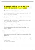
Population variance
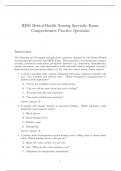
Sample variance
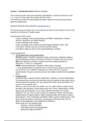
Standard deviation
Standard deviation relating an individual to a population.
Standard error relating a sample to a population.
Conditional indexing:
Tmp <- dat[dat$gender == “M”, ]
Tmp <- dat[dat$gender == “M”& dat$study == “IS”, ] combining conditions.
Tmp <- dat[dat$gender != “M” | dat$english_grade > 7, ] not equal to.
Adding new columns:
Dat$diff <- dat$english_grade – dat$english_score.
Head() the first 6 lines of the data.
Str() the structure of the data.
Barplot: visualizes nominal data.
Table()
Barplot(table())
Hist() shows frequency of all values in groups. Looks for a general pattern, symmetry, outliers.
Col = c kleuren voor de barplot.
Ylim = c limiet voor de y-as.
Main naam voor de barplot.
Xlab naam voor de x-as.
Ylab naam voor de y-as.
Descriptive statistics:
Mean() mean for the variable.
Min() minimum value.
Max() maximum value.
Range() gives both min and max.
Diff() gives difference between max and min.
Var() variance: average squared deviation form mean.
Sd() standard deviation (square root of variance).
Table(dat$gender) frequency table.
Table(dat$gender, dat$study) cross table.
Lecture & lab 2:
Descriptive statistics:
- Describes data.
- Measures of central tendency mean, median, mode.
- Measures of variation range, IQR, variance, standard deviation.
o Information on distribution of the data.
Inferential statistics:
- Describes data of sample to infer patterns in population statistical tests.
- Generalize outcomes of a sample to a population.
o Compares 2 groups (or a single group with fixed value).
o Associations between 2 variables.
Categorical variables:
- Nominal just categorization, no ordering (gender).
- Ordinal categories have order, but do know distance (bad - neutral – good).
Numerical variables:
- Interval numbered categories have a known distance between them (degrees Celsius).
, - Ratio numbered categories with a meaningful 0 (age).
Density curve:
- Visualizes a distribution.
o Plot(density(), main =, xlab = )
Central tendency:
Mode most frequent (all measurement levels).
Median middle value of sorted data (ordinal, interval, ratio).
Mean sum of observations divided by number of observations (interval & ratio).
Measure of variation:
Quartiles 4 subsets of equal size. Quantile().
- Q1 cutpoint between group 1 and 2 (first 25%).
- Q2 cutpoint between group 2 and 3 (first 50%).
- Q3 cutpoint between group 3 and 4 (first 75%).
Percentiles hundred equal-sized subsets.
- Q1 = 25th percentile.
- Q2 = 50th percentile.
Interquartile range IQR() = Q3-Q1.
Visualization of variation boxplot (visualizes numerical data).
Important measures of variation:
Population variance
Sample variance
Standard deviation
Standard deviation relating an individual to a population.
Standard error relating a sample to a population.