Exercise 35, Calculating Pearson Chi-Square
1. Do the example data in Table 35-2 meet the assumptions for the Pearson chi
square test? Provide a rationale for your answer.
a. Yes, the assumptions are met for the chi-square test.
b. There is only one datum entry for each participant, the variable are at nominal level
and each category is mutually exclusive and exhaustive.
2. Compute the chi square test. What is the chi square value?
a. 51.938
3. Is this chi square significant at alpha=0.05? Show how you arrived at your answer.
a. Per the table provided, the significance is 0.000, therefore the chi squared is
significant as it is below the set alpha of 0.05
4. Is using SPSS, what is the exact likelihood of obtaining the chi square value at
least as extreme as or as close to the one that was actually observed, assuming that the null
hypothesis is true?
a. The exact likelihood is 1%, assuming the null hypothesis is true
5. Using the numbers in the contingency table, calculate the percentage of antibiotic users who
tested positive for candiduria.
a. 15/58=0.258*100=26%
6. Using the numbers in the contingency table, calculate the percentage of non- antibiotic users
who tested positive for candiduria.
a. 0/39=0%
,7. Using the numbers in the contingency table, calculate the percentage of veterans with
candiduria who had a history of antibiotic use.
a. 15/15=1*100=100%
8. Using the numbers in the contingency table, calculate the percentage of veterans with
candiduria who had no history of antibiotic use.
a. 0/15=0%
9. Write your interpretation of the results as you would in an APA-formatted journal.
a. A Pearson chi-square analysis indicated that antibiotic users had
a significantly higher rate of candiduria than those who did not use antibiotics, chi-
square (1)= 51.938, p=0.000. These findings suggest that antibiotic use may be a risk
factor for candiduria development and further researcher is needed to investigate
candiduria as a direct effective of antibiotic use.
10. Was the sample size adequate to detect differences between the two groups
in this example? Provide a rationale for your answer.
a. The sample size was adequate to detect a different between the two groups, because a
significant difference was found, p=0.000, which is smaller than alpha=0.05
Part 1
After following the steps to obtain a 2x2 table (also known as “cross tabulation”) crossing binge
with depression the results are illustrated below. Using the data from the cross tabulation the odds
ratio for depression among those exposed to binge drinking is as follow.
, Odds Ratio = a/b = a x d = 1,275x550 = 701,250 = 0.983 c/d bxc 5,441x131 712,771
Therefore, the odds ratios would is interpreted as being a good estimate of the relative risk
because which means it unchanged.
Ever told you that you have a
depre ssive disor der, inclu ding depre ssion, major depre ssion, dysth ymia, or minor depre
ssion (ADD EPE V2)
No
No value Yes No Total
value
Calculated variable for binge drinkers, men having 5+
drinks on one occasion and women having 4+ drinks on
one occasion (_RFBING5)
No val ue
1. Do the example data in Table 35-2 meet the assumptions for the Pearson chi
square test? Provide a rationale for your answer.
a. Yes, the assumptions are met for the chi-square test.
b. There is only one datum entry for each participant, the variable are at nominal level
and each category is mutually exclusive and exhaustive.
2. Compute the chi square test. What is the chi square value?
a. 51.938
3. Is this chi square significant at alpha=0.05? Show how you arrived at your answer.
a. Per the table provided, the significance is 0.000, therefore the chi squared is
significant as it is below the set alpha of 0.05
4. Is using SPSS, what is the exact likelihood of obtaining the chi square value at
least as extreme as or as close to the one that was actually observed, assuming that the null
hypothesis is true?
a. The exact likelihood is 1%, assuming the null hypothesis is true
5. Using the numbers in the contingency table, calculate the percentage of antibiotic users who
tested positive for candiduria.
a. 15/58=0.258*100=26%
6. Using the numbers in the contingency table, calculate the percentage of non- antibiotic users
who tested positive for candiduria.
a. 0/39=0%
,7. Using the numbers in the contingency table, calculate the percentage of veterans with
candiduria who had a history of antibiotic use.
a. 15/15=1*100=100%
8. Using the numbers in the contingency table, calculate the percentage of veterans with
candiduria who had no history of antibiotic use.
a. 0/15=0%
9. Write your interpretation of the results as you would in an APA-formatted journal.
a. A Pearson chi-square analysis indicated that antibiotic users had
a significantly higher rate of candiduria than those who did not use antibiotics, chi-
square (1)= 51.938, p=0.000. These findings suggest that antibiotic use may be a risk
factor for candiduria development and further researcher is needed to investigate
candiduria as a direct effective of antibiotic use.
10. Was the sample size adequate to detect differences between the two groups
in this example? Provide a rationale for your answer.
a. The sample size was adequate to detect a different between the two groups, because a
significant difference was found, p=0.000, which is smaller than alpha=0.05
Part 1
After following the steps to obtain a 2x2 table (also known as “cross tabulation”) crossing binge
with depression the results are illustrated below. Using the data from the cross tabulation the odds
ratio for depression among those exposed to binge drinking is as follow.
, Odds Ratio = a/b = a x d = 1,275x550 = 701,250 = 0.983 c/d bxc 5,441x131 712,771
Therefore, the odds ratios would is interpreted as being a good estimate of the relative risk
because which means it unchanged.
Ever told you that you have a
depre ssive disor der, inclu ding depre ssion, major depre ssion, dysth ymia, or minor depre
ssion (ADD EPE V2)
No
No value Yes No Total
value
Calculated variable for binge drinkers, men having 5+
drinks on one occasion and women having 4+ drinks on
one occasion (_RFBING5)
No val ue