Outliers
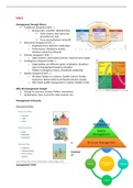
Replace outliers = 1 if abs(z)>=4 & z<.
Or 3 if it is a normal distribution
Extra
Gen x = y>2 | y2>4
X= 1 when y>2 or y2>4
Table factor A factor B, c(mean var) gives mean of the variable for each group
Combine L1, L2, L3 into L4: mat L4 = (L1/L2/L3)
Check for homogeneity:
Robvar var, by(groups) H0 = heterogeneity
One-way ANOVA
Anova x var##var Gives full-factorial design (all interactions)
Postestimation:
- estat esize gives eta2
- Pwmean var, over(groups) Shows how groups differ
- Margins y, noestimcheck noestimcheck needed with repeated measures
marginsplot Check direction effect y
One-way repeated measures ANOVA
First it should be in a long format Reshape long var, i(id) j(condition)
anova x y1/y1#id y2/y2#id y1#y2 id, repeated(y1 y2)
Mixed ANOVA
Between factor y1 en y2 en within t
anova x y1#y2/id|y2#y1 t t#y1 t#y2 t#y1#y2, repeated(t)
Analysis of covariance
2 extra assumptions regarding covariate:
- Linearity between covariate and dependent variable:
inspect scatterplot
- Regression slopes for covariate on the dependent variable same for each group.
First run regression equation as intended but add all interactions with covariate. If
there is a significant interaction, if it is different for different factors.
, Simple linear regression
Create dummy variables of y tab y, gen(dummy)
Reg x i.y i. also creates dummy variables for y
Postestimation after reg to test if dummy 1 is different from dummy 2:
Test_b[2.y] = _b[4.y]
Or run another regression and leave another category out as reference category.
Regression assumptions:
1. Standardized residuals are normally distributed:
predict e, rstandard
hist e, norm
skest e / swilk e
2. Linearity / homoscedasticity plotting residuals against predicted values.
predict y, xb
scatter e y
inspect plot
3. Check outliers:
a. Leverage points: outlier when higher than critical value 3(k+1)/n
k number of predictors
n sample size
predict lev, leverage
list id lev if lev > 3(k+1)/n
b. Z-scores:
List id e if abs(e)>3
c. Influential data points (cooksd should not be larger than 1)
predict cooksd, cooksd
list id cooksd if cooksd >1
Gen outliers = (lev>3(k+1)/n) | abs(e)>3 | cooksd>1)
If heterogeneity is still a problem use a robust regression:
Reg x y, vce(hc3)
Multiple regression = Multiple regression is very similar to simple regression, except that in
multiple regression you have more than one predictor variable in the equation.
Multicollinearity:
1. Look at pwcorr x1 x2, sig
(should not have large correlations >0.6)
2. Run regression and then vif.
issue when average vif > 2.5 or single>10.
Pcorr: partial and semi partial correlation
(semi partial correlation)2 = variance in x uniquely explained by y.
Stein corrected R-squared average: r2 taken from many samples of the same population.
Calculate by hand.
n−1 n−2 n+1
ρ^ 2c =1−( )( )( )(i−R 2)
n−k−1 n−k −2 n
Predict x for another sample based on regression model of the old sample
Gen a new variable and compute the predicted value by typing in the regression equation.
Hireg determine whether added predictors lead to a statistically significant increase in R2.

