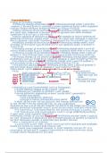
Tree-based methods for regression and classification involve stratifying/segmenting the
predictor space into a number of simple regions.
For prediction, we use mean/mode response value for the training observations in the region
to which they belong.
Decision tree: the set of splitting rules to segment the predictor summarized in a tree
8.1: The basics of decision trees
8.1.1 Regression trees
In the tree analogy, decision trees are typically drawn upside down.
Splitting rule: starting at the top of the tree.
For every observation fall into each region, we make the same prediction: mean of the response
values for the training observation in each region
Decision tree: Superfical similarities with KNN
- K-NN is expensive because each prediction requires a comparison to entire training set.
- What is we partitioned the training set ahead of time, summarized the partitions with
simple rules, and pre-calculated predictions?
Purpose
Partition feature space into regions where values of target variables are relatively
homogeneous(or pure if classification tree case)
Decision tree terminologies
Terminal nodes/leaves = Regions: where all observations end up.
Internal nodes = Points along the tree where the predictor space is split
- The first internal node with the most important factor to determine the response factor
, Value at the top in the square = predicted y value
Advantage:
- Interpretability
- Similarity to human decisions
- No dummy variable required
- Good “Base learners”
- It can be visually and intuitively displayed
- Easy to handle qualitative predictors without creating dummy variables
- Can deal with the non-linear relationship by digging into specific features multiple times
in splitting
Disadvantage
- Not competitive in terms of accuracy (aggregation of trees can improve it)
- Trees can be very non-robust: small change in the data can cause a large change in the
final estimated tree
Process: Greedy approach
It is computationally infeasible to consider every possible partition of the feature space into J
boxes.
In creation of the decision tree, we take top-down greedy approach/recursive binary
splitting (for decision tree case)
o It begins at the top of the tree and then successively splits the predictor space
with two new branches
o It is greedy as the best split is made at the each of the split rather than looking
ahead and picking one that lead to a better tree in some future step.
Example: predicting salary of baseball players
1. Years <4.5?
2. For players with years <4.5, find the mean response value for those players (e.g. mean
log salary of 5.107 = $165,174)

