SUMMARY TRANSPORT ECONOMICS & MANAGEMENT
HC 1
The economics of demand
Demand analysis: conceptual framework to describe preference.
- Demand; willingness-to-pay (determines revenues)
- Each user (rail freight company, cargo owner) has its own set of preferences.
Assumptions: consumer
- Is rational
- Is self-interested
- Maximizes utility U
Consumer makes a choice to buy good Q1 or Q2 (e.g. options on your car), given his/her budget constraint: Y=p1 Q1
+ p2 Q2
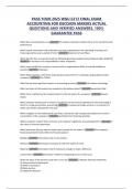
Indifference curve: combinations of X1 or X2 that yield the same utility level
Interpretation of (inverse) demand curve:
- in the optimum (point D): slope budget
curve = slope indifference curve; p1/p2
=∆Q2/ ∆Q1
- Inverse demand: p1=p2*∆Q2/∆Q1
o Maximum price we are willing
to pay (and a company can
charge) so that our utility is still
maximized.
o The ‘benefit’ we derive from
Q1 (expressed in monetary
terms): often used as measure
of welfare (as used in cost-benefit analysis)
o Measures how much (value) of Q2 is given up for more Q1, given that utility is maximized
,What determines demand?
• Price of substitutes ‘standard’ variables not necessarily
• Price of complementary goods controlled by you as a manager
• Income
• Population
• Bureaucracy determinants of transport demand
• Security also not under control by manager
• Popularity/image
• Speed determinants of transport under control
• Reliability by manager: part of planning process
Elasticity of demand
- Elasticity: responsiveness of demand to change a factor (e.g. price), measured in percentages
- Price elasticity of demand: % change in output / % change in price
o ∆X = change in variable X: ∆X= Xnew – X
o % change in price = (Pnew-P)/P = ∆P/P
o % change in output = (Qnew – Q)/Q = ∆Q/Q
∆Q/Q ∆Q 𝑃
- Price elasticity of demand: ∆P/P = ∆P × 𝑄
- Point-elasticity: measured in a point (infinitesimal price change ∂P)
o The elasticity at the current level of demand
∂Q 𝑃
o Price elasticity then is: ∂P × 𝑄
o For instance, a price elasticity of -1.15
means that demand decreases by 1.15%
if the price increases by 1%
o Inelastic demand: -1 < price elasticity < 0
o Elastic demand: price elasticity <-1
Determinants of elasticities
Price elasticity influenced by:
• Proportion of consumer expenditure: misschien is
een waterflesje op de VU heel duur maar het is
maar een klein deel van je totale uitgaven in het
dagelijks leven
• Addictiveness: cigarets
• Level of necessity: hoe hard heb je het nodig?
• Time scale: als je iets snel nodig hebt kijk minder snel naar de prijs. → inelastisch Als je iets van over 10
weken nodig hebt kijk je meer naar de prijs → meer elastisch.
• Availability of substitutes
Welfare
Consumers
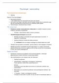
- Inverse demand curve gives willingness-to-pay
o Benefit consumer(s) derive(s) from additional good
o Area under inverse demand curve measures total benefit or total surplus
,Estimating demand
- Need for info on demand
parameters
o elasticities
- Q = f(P,Y,t)
o Demand (Q) is a
function of price P, income Y, and time trend t.
o Q=α*P+β*Y+γ*t or lnQ=α*lnP+β*lnY+γ*t
- Assumes a causal relation between variables
o P, Y and t ‘cause’ Q
o Data on prices, demand, income and other characteristics needed
- Part of tutorial
o Time series
o OLS
HC 2
Factors of production for transport company
- Land (raw materials) e.g. fuel
- Labor e.g. drivers
- Capital (man-made resources) e.g. trucks
o Machines
o Computer systems
o Financial capital
- Entrepreneurship e.g. ownership/management
o Risk-taking; organization to other factors
Cost functions
Choose production factors so that costs are minimized
- Produce output Q (e.g. Q = δLα K β : Cobb-Douglas production function)
- Use e.g. production factors
o Labour L at price w
o Capital K at price r
o α and β are the weights of capital and labor in the production function
- Minimize: C= w*L + r*K
o Subject to: target level Q can be produced from (K, L)
- Cost function C=C(Q,r,k): minimum cost of producing Q given input prices, using optimal levels of (K,L). in
other words: all combinations of inputs (labour and capital) which gives you always the lowest cost for a
certain amount of Q.
Cost minimization: slope iso-cost = slope isoquant r/w=∆L/∆K
, Cost function requirements:
- Increasing in Q
- Non-decreasing in w,r
- C(Q,x*w,x*r) = x*C(Q,w,r)
- Application of cost function (implicitly) assumes cost
minimization (except for governments issues for
instance when speed is more important)
o Rational behaviour and self-interest
Costs
- Fixed costs: are costs that remain the same
regardless of the output that is produced.
- Variable costs: are costs that change as the level of output changes.
o Outsourcing transforms fixed into variable costs.
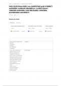
- Marginal costs: change in TC (VC) resulting from a unit (infinitesimal) change in output
o ∂TC/∂Q; TC=total cost, Q=output
• Average fixed costs: not a straight line because it is the average fixed cost so it is divided by Q.
• Marginal cost line should always cross the minimum of the AVC or AFC
2 ways to calculate the Total cost:
• Total cost line = AVC x Q
• Add all the additional cost together (MC) is also the total cost. Area under MC curve until a certain amount
of Q is the total cost.
1 calculate total cost
2 calculate total cost
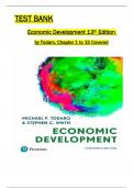
Economies of scale
- Cost function: C(Q,w,r)
- Average cost (AC): C/Q
- Marginal cost (MC): ∂C/∂Q
HC 1
The economics of demand
Demand analysis: conceptual framework to describe preference.
- Demand; willingness-to-pay (determines revenues)
- Each user (rail freight company, cargo owner) has its own set of preferences.
Assumptions: consumer
- Is rational
- Is self-interested
- Maximizes utility U
Consumer makes a choice to buy good Q1 or Q2 (e.g. options on your car), given his/her budget constraint: Y=p1 Q1
+ p2 Q2
Indifference curve: combinations of X1 or X2 that yield the same utility level
Interpretation of (inverse) demand curve:
- in the optimum (point D): slope budget
curve = slope indifference curve; p1/p2
=∆Q2/ ∆Q1
- Inverse demand: p1=p2*∆Q2/∆Q1
o Maximum price we are willing
to pay (and a company can
charge) so that our utility is still
maximized.
o The ‘benefit’ we derive from
Q1 (expressed in monetary
terms): often used as measure
of welfare (as used in cost-benefit analysis)
o Measures how much (value) of Q2 is given up for more Q1, given that utility is maximized
,What determines demand?
• Price of substitutes ‘standard’ variables not necessarily
• Price of complementary goods controlled by you as a manager
• Income
• Population
• Bureaucracy determinants of transport demand
• Security also not under control by manager
• Popularity/image
• Speed determinants of transport under control
• Reliability by manager: part of planning process
Elasticity of demand
- Elasticity: responsiveness of demand to change a factor (e.g. price), measured in percentages
- Price elasticity of demand: % change in output / % change in price
o ∆X = change in variable X: ∆X= Xnew – X
o % change in price = (Pnew-P)/P = ∆P/P
o % change in output = (Qnew – Q)/Q = ∆Q/Q
∆Q/Q ∆Q 𝑃
- Price elasticity of demand: ∆P/P = ∆P × 𝑄
- Point-elasticity: measured in a point (infinitesimal price change ∂P)
o The elasticity at the current level of demand
∂Q 𝑃
o Price elasticity then is: ∂P × 𝑄
o For instance, a price elasticity of -1.15
means that demand decreases by 1.15%
if the price increases by 1%
o Inelastic demand: -1 < price elasticity < 0
o Elastic demand: price elasticity <-1
Determinants of elasticities
Price elasticity influenced by:
• Proportion of consumer expenditure: misschien is
een waterflesje op de VU heel duur maar het is
maar een klein deel van je totale uitgaven in het
dagelijks leven
• Addictiveness: cigarets
• Level of necessity: hoe hard heb je het nodig?
• Time scale: als je iets snel nodig hebt kijk minder snel naar de prijs. → inelastisch Als je iets van over 10
weken nodig hebt kijk je meer naar de prijs → meer elastisch.
• Availability of substitutes
Welfare
Consumers
- Inverse demand curve gives willingness-to-pay
o Benefit consumer(s) derive(s) from additional good
o Area under inverse demand curve measures total benefit or total surplus
,Estimating demand
- Need for info on demand
parameters
o elasticities
- Q = f(P,Y,t)
o Demand (Q) is a
function of price P, income Y, and time trend t.
o Q=α*P+β*Y+γ*t or lnQ=α*lnP+β*lnY+γ*t
- Assumes a causal relation between variables
o P, Y and t ‘cause’ Q
o Data on prices, demand, income and other characteristics needed
- Part of tutorial
o Time series
o OLS
HC 2
Factors of production for transport company
- Land (raw materials) e.g. fuel
- Labor e.g. drivers
- Capital (man-made resources) e.g. trucks
o Machines
o Computer systems
o Financial capital
- Entrepreneurship e.g. ownership/management
o Risk-taking; organization to other factors
Cost functions
Choose production factors so that costs are minimized
- Produce output Q (e.g. Q = δLα K β : Cobb-Douglas production function)
- Use e.g. production factors
o Labour L at price w
o Capital K at price r
o α and β are the weights of capital and labor in the production function
- Minimize: C= w*L + r*K
o Subject to: target level Q can be produced from (K, L)
- Cost function C=C(Q,r,k): minimum cost of producing Q given input prices, using optimal levels of (K,L). in
other words: all combinations of inputs (labour and capital) which gives you always the lowest cost for a
certain amount of Q.
Cost minimization: slope iso-cost = slope isoquant r/w=∆L/∆K
, Cost function requirements:
- Increasing in Q
- Non-decreasing in w,r
- C(Q,x*w,x*r) = x*C(Q,w,r)
- Application of cost function (implicitly) assumes cost
minimization (except for governments issues for
instance when speed is more important)
o Rational behaviour and self-interest
Costs
- Fixed costs: are costs that remain the same
regardless of the output that is produced.
- Variable costs: are costs that change as the level of output changes.
o Outsourcing transforms fixed into variable costs.
- Marginal costs: change in TC (VC) resulting from a unit (infinitesimal) change in output
o ∂TC/∂Q; TC=total cost, Q=output
• Average fixed costs: not a straight line because it is the average fixed cost so it is divided by Q.
• Marginal cost line should always cross the minimum of the AVC or AFC
2 ways to calculate the Total cost:
• Total cost line = AVC x Q
• Add all the additional cost together (MC) is also the total cost. Area under MC curve until a certain amount
of Q is the total cost.
1 calculate total cost
2 calculate total cost
Economies of scale
- Cost function: C(Q,w,r)
- Average cost (AC): C/Q
- Marginal cost (MC): ∂C/∂Q