Biostatistics 2 2022 Lecture 1 Feb 7 2022
Chechk residuals
Nominal data -> no order in data (aka no factors in R)
e.g. sex
Ordinal data -> ordered but diffs between values important
e.g. hotel rating
interval data -> ordered, zero point arbitrary
differences make sense but ratios do not
e.g. temperature in degrees
ratio -> ordered, natural zero point
e.g. height
discrete -> can only take certain values, e.g. dead/alive, species, number of cells
continuous -> can take any value (within certain range), e.g. weight speed, concentration
Discrete data -> use a bar plot, with frequencies and relative frequencies (added all frequencies must
be 1)
Continuous data -> make different categories and use a histogram with the different ranges next to
each other. Bin/class width means the size of the group ranges.
Population -> e.g. all students at RUG, whole population
Sample -> e.g. 200 randomly selected students at RUG, a part of the population
Population size N, sample size n
population mean -> sum of all the values divided by N
sample mean -> sum of the sample of the population divided by n, this is the estimate for the
population mean. If the sample size is large enough it comes pretty close to the population mean
mode -> most frequently occurring value (or class)
median -> central value when data are ranked (n+1)/2. First rank the values, when there are even
numbers take the two central numbers and divide them by 2
The median is less sensitive to outliers than the (arithmetic) mean. Because the mean is influenced
by a long tail, then the mean is not useful.
,0.5 quantile or 50th percentile = Q2 or median
q quantile or 100qth percentile: a proportion q of data has smaller value
0.7 quantile or 70th percentile: 0.7 (70%) of data has smaller value
Measures of variation, small variation -> small deviation from the mean. Large variation -> large
deviation from the mean.
Unit of the variance is kg^2
Unit of the standard deviation
Coefficient of variation has no unit, unitless. You can compare this value easily between different
studies, because you can compare studies with different units, because the coefficient of variation
has no unit.
Range -> highest minus lowest values
Inter-quartile range (IQR) = Q3-Q1
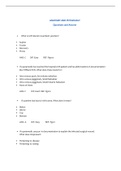
Box is the middle part of the plot, the inter-quartile range. The whiskers indicate the lower quartile
and the upper quartile, except when there are numbers that are more than 1.5 box away from the
median (indicated with stars). These are outliers far away from the median.
Discrete probability distributions
- Random variable Y can only take discrete values (i.e. integers, in practice usually larger or
equal to 0)
- Each possible value k of Y has a probability Pr(Y=k)
- The probabilities of all possible values sum to 1
,Uniform distribution
- All possible values of Y equally likely
- Throw of a coin for example
Binomial distribution
- Nr of “successes” in n independent “Bernoulli” trials each with same probability of success p
- Has two parameters
- Expected number of successes is n*p
- Variance is n*p(1-n)
Poisson distribution
- Non-negative counts: nr of “random” events per fixed amount of time or space
- E.g. number of trees struck by lightning per acre of forest
- Single parameter
Goodness of fit tests
Test whether our data is reasonable
See how well observed frequencies match expected frequencies
How well do our observed data fit to a hypothetical (discrete) probability distribution?
Hypothesis testing
Test procedure
1. Formulate H0 and Ha
2. Choose test
3. Calculate test statistic and compare value to its probability distribution
4. Determine P-value associated with value of test statistic or one more extreme (given H0 true)
5. Reject H0 if P< α ; retain H0 otherwise
P-value: probability of observed data (or more extreme result) given H0 is true
Chi-square GOF test
- If observed similar to expected, X^2 small
- If observed very different from expected, X^2 large
- If H0 true, X^2 approximately follows X^2 distribution for K-1 degrees of freedom, but most
of the time K-2 degrees of freedom
- Look up p-value in X^2 tables for K-1 d.f.
- Reject H0 if p<0.05; otherwise retain H0
- Important requirements; raw counts, not percentages
- No more than 20% expected counts < 5, and none < 1
- Fisher’s exact test for 2x2 tables
- Otherwise combine (pool) categories
R gives exact p-values
Chisq.test(c(189,91), p=c(3/4, ¼)
Continuous probability distributions
- Random variable Y take continuous real values
- Y has a probability density, probability that the value is between an interval
- The probability densities integrate to 1
, Uniform distribution
- All outcomes equally likely (between limits)
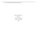
Normal distribution
- Standard normal distribution, mean of 0 and variance of 1
- For any normal distribution, there is a 95% probability that a random draw from that
distribution is within 2 standard deviations from the mean. Within 1 standard deviation from
the mean is about 69% and 3 standard deviation is about 99%
- Test whether a sample is drawn from a normal distribution
- Use Q-Q plots
y <- rnorm(n=100,mean=0,sd=1) #100 normal random numbers
hist(y) #histogram
qqnorm(y) #draw QQ plot without line
qqline(y) # add line
If the points are sufficiently close to the line, the assumption that the data is from a normal
distribution is reasonable.
Chi-squared distribution
y <- rchisq(n=100, df=1) #100 chisq random numbers
hist(y) #histogram
qqnorm(y, pch=16,main=””) #draw QQ plot without line
qqline(y) # add line
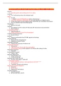
t-distribution
y <- rt(n=100,mean=0,df=2) #100 t random numbers
hist(y) #histogram
qqnorm(y) #draw QQ plot without line
qqline(y) # add line
- Has further tails
Test for normality: Shapiro- Wilk
y <- rnorm(n=100, mean=0, sd=1) #100 normal random numbers
shapiro.test(y)
Big p-value means that the H0, that the data is drawn from a normal distribution, should not be
rejected.
Chechk residuals
Nominal data -> no order in data (aka no factors in R)
e.g. sex
Ordinal data -> ordered but diffs between values important
e.g. hotel rating
interval data -> ordered, zero point arbitrary
differences make sense but ratios do not
e.g. temperature in degrees
ratio -> ordered, natural zero point
e.g. height
discrete -> can only take certain values, e.g. dead/alive, species, number of cells
continuous -> can take any value (within certain range), e.g. weight speed, concentration
Discrete data -> use a bar plot, with frequencies and relative frequencies (added all frequencies must
be 1)
Continuous data -> make different categories and use a histogram with the different ranges next to
each other. Bin/class width means the size of the group ranges.
Population -> e.g. all students at RUG, whole population
Sample -> e.g. 200 randomly selected students at RUG, a part of the population
Population size N, sample size n
population mean -> sum of all the values divided by N
sample mean -> sum of the sample of the population divided by n, this is the estimate for the
population mean. If the sample size is large enough it comes pretty close to the population mean
mode -> most frequently occurring value (or class)
median -> central value when data are ranked (n+1)/2. First rank the values, when there are even
numbers take the two central numbers and divide them by 2
The median is less sensitive to outliers than the (arithmetic) mean. Because the mean is influenced
by a long tail, then the mean is not useful.
,0.5 quantile or 50th percentile = Q2 or median
q quantile or 100qth percentile: a proportion q of data has smaller value
0.7 quantile or 70th percentile: 0.7 (70%) of data has smaller value
Measures of variation, small variation -> small deviation from the mean. Large variation -> large
deviation from the mean.
Unit of the variance is kg^2
Unit of the standard deviation
Coefficient of variation has no unit, unitless. You can compare this value easily between different
studies, because you can compare studies with different units, because the coefficient of variation
has no unit.
Range -> highest minus lowest values
Inter-quartile range (IQR) = Q3-Q1
Box is the middle part of the plot, the inter-quartile range. The whiskers indicate the lower quartile
and the upper quartile, except when there are numbers that are more than 1.5 box away from the
median (indicated with stars). These are outliers far away from the median.
Discrete probability distributions
- Random variable Y can only take discrete values (i.e. integers, in practice usually larger or
equal to 0)
- Each possible value k of Y has a probability Pr(Y=k)
- The probabilities of all possible values sum to 1
,Uniform distribution
- All possible values of Y equally likely
- Throw of a coin for example
Binomial distribution
- Nr of “successes” in n independent “Bernoulli” trials each with same probability of success p
- Has two parameters
- Expected number of successes is n*p
- Variance is n*p(1-n)
Poisson distribution
- Non-negative counts: nr of “random” events per fixed amount of time or space
- E.g. number of trees struck by lightning per acre of forest
- Single parameter
Goodness of fit tests
Test whether our data is reasonable
See how well observed frequencies match expected frequencies
How well do our observed data fit to a hypothetical (discrete) probability distribution?
Hypothesis testing
Test procedure
1. Formulate H0 and Ha
2. Choose test
3. Calculate test statistic and compare value to its probability distribution
4. Determine P-value associated with value of test statistic or one more extreme (given H0 true)
5. Reject H0 if P< α ; retain H0 otherwise
P-value: probability of observed data (or more extreme result) given H0 is true
Chi-square GOF test
- If observed similar to expected, X^2 small
- If observed very different from expected, X^2 large
- If H0 true, X^2 approximately follows X^2 distribution for K-1 degrees of freedom, but most
of the time K-2 degrees of freedom
- Look up p-value in X^2 tables for K-1 d.f.
- Reject H0 if p<0.05; otherwise retain H0
- Important requirements; raw counts, not percentages
- No more than 20% expected counts < 5, and none < 1
- Fisher’s exact test for 2x2 tables
- Otherwise combine (pool) categories
R gives exact p-values
Chisq.test(c(189,91), p=c(3/4, ¼)
Continuous probability distributions
- Random variable Y take continuous real values
- Y has a probability density, probability that the value is between an interval
- The probability densities integrate to 1
, Uniform distribution
- All outcomes equally likely (between limits)
Normal distribution
- Standard normal distribution, mean of 0 and variance of 1
- For any normal distribution, there is a 95% probability that a random draw from that
distribution is within 2 standard deviations from the mean. Within 1 standard deviation from
the mean is about 69% and 3 standard deviation is about 99%
- Test whether a sample is drawn from a normal distribution
- Use Q-Q plots
y <- rnorm(n=100,mean=0,sd=1) #100 normal random numbers
hist(y) #histogram
qqnorm(y) #draw QQ plot without line
qqline(y) # add line
If the points are sufficiently close to the line, the assumption that the data is from a normal
distribution is reasonable.
Chi-squared distribution
y <- rchisq(n=100, df=1) #100 chisq random numbers
hist(y) #histogram
qqnorm(y, pch=16,main=””) #draw QQ plot without line
qqline(y) # add line
t-distribution
y <- rt(n=100,mean=0,df=2) #100 t random numbers
hist(y) #histogram
qqnorm(y) #draw QQ plot without line
qqline(y) # add line
- Has further tails
Test for normality: Shapiro- Wilk
y <- rnorm(n=100, mean=0, sd=1) #100 normal random numbers
shapiro.test(y)
Big p-value means that the H0, that the data is drawn from a normal distribution, should not be
rejected.