Inhoudsopgave
Notes Inferential Statistics – Test 1 ....................................................................................................................... 2
Self-Study B: the normal model + finding probabilities ...................................................................................... 2
Lecture 1: Introduction to statistical inference. Sampling Distribution Model for A PROPORTION and
Confidence intervals for PROPORTIONS........................................................................................................... 8
Statistical inference and the fundamental problem of uncertainty in statistics ............................................... 8
Sampling distribution model FOR PROPORTIONS (theory + assumptions) ................................................... 10
Using the theory about the Sampling Distribution Model for PROPORTIONS (theoretical examples, canvas
page 1.1: ex1 (first year student), ex3 + ex4) .................................................................................................... 13
5. Using the theory about the Sampling Distribution Model for PROPORTIONS in practice: → Confidence
interval for a proportion .................................................................................................................................... 15
1.1: Sampling distribution model for proportions ............................................................................................. 17
Exercises 1.1 Canvas ......................................................................................................................................... 17
1.2: Confidence intervals for proportions .......................................................................................................... 19
Exercises 1.2 Canvas ......................................................................................................................................... 19
Lecture 2: Inference about one mean: Confidence intervals (SDM + CLT + TEST) .................................... 23
Sampling distribution model for a mean............................................................................................................ 23
Inference for means: confidence interval for a mean ........................................................................................ 26
2.1: Sampling distribution model for means (SDM + CLT + TEST) .............................................................. 29
Exercises Canvas ............................................................................................................................................... 29
2.2: Confidence interval for a mean .................................................................................................................... 33
Exercises Canvas ............................................................................................................................................... 35
Reflection Session 1: CI Proportions and Means .............................................................................................. 39
Lecture 3: Inference for means – Test for one mean......................................................................................... 45
Inference for means: hypothesis test for one mean............................................................................................ 45
An example of the one sample t-test................................................................................................................... 48
So an conclusion / overview t-procedure for the one sample situation: ............................................................ 55
Lecture 3B: More about tests .............................................................................................................................. 56
Interpretation of outcomes (statistical significance, magnitude (grootte) of the outcome and practical
significance) ....................................................................................................................................................... 56
Investigating normality: Descriptive + Shapiro-Wilk test................................................................................. 57
More about assumptions and an alternative solution (when to use the Sign test)............................................. 60
Canvas Lecture 3B: more about tests – part II.................................................................................................. 61
1
,3.1: Steps in performing a statistical test ............................................................................................................ 68
3.2: Exercises One-Sample t-test ......................................................................................................................... 69
3.3: Exercises More about Tests .......................................................................................................................... 82
Notes Inferential Statistics – Test 1
Self-Study B: the normal model + finding probabilities
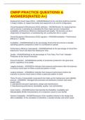
Normal model = N(mu, sigma)
Standard normal model (or: Z-distribution) = N(0,1)
Exercises via the distribution of IQ-scores
Assume: normal distribution
- Mean = 100
- SD = 16
→ IQ has a N(100, 16)-distribution
1. What percentage of observations is expected to fall within one standard deviation
from the mean and what are the borders of that interval?
→ 68% of values fall within 1 SD from the mean
→ 68% of the values fall between: 100 – 16 = 84 & 100 + 16 = 116
2. What percentage of observations is expected to fall within two standard deviations
from the mean and what are the borders of that interval?
→ 95% of values fall within 2 SD from the mean
→ 95% of the values fall between: 100 – 32 = 68 & 100 + 32 = 132
3. What is the expected proportion that has at least a score of 132 or more on the IQ-
scale?
→ IQ-score of 132 is at least 2 SD away from the mean.
→This means that 100 – 95 = 5% / 2 = 2,5% has at least a score of 132 or more.
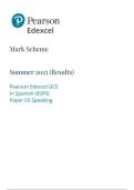
Using the N(0, 1)-distribution and reading the z-table
Calculating z-scores by:
(observation – mean of population (mu) ) / SD (sigma)
Proportions on Z-table = part below
1 - proportions on Z-table = part above
4. How big is the group with an IQ-score of 124 or more? (What is the expected
proportion that has at least a score of 124 or more on the IQ-scale?)
▪ 4a. What is the standardized score, the z-value, for the IQ-score 124?
→ 124 – 100 (mean) / 16 (SD) = 1.5
▪ 4b. What is the expected proportion that has at least a score of 124 or more on the IQ-
scale? (assuming a normal model)
2
, (use Z-table with Standardized Normal Probabilities)
→ So P(Z > 1.5) = ?
→ In the Z-table you see when Z is 1.5, the SNP is .9332.
→ Expected proportion that has 124+ IQ = 1 – 0.9332 = 0.0668 = 6.68%
Other examples
- What percent of a standard normal model is found for: z < 2.25?
→ .9878 (see Z-table) = 98.78%
- What percent of a standard normal model is found for: -1 < z < 1.15?
→ 1.15 = .8749 & -1 = .1587
→ .8749 - .1587 = .7162 = 71.62%
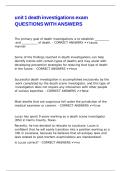
- Reversing the problem. How can we find the z-value for a certain cumulative
probability?
o What is the value of Z for the highest 75%? →
100 – 75 = 25% = 0,2500.
Z-table says .2514 is closest, so Z-score = -.67
Z-table says there are two values near the probability of .9500, namely .9495 with a Z-
value of 1.64 & .9505 with a Z-value of 1.65. --> We take the z-value in between:
1.645
Specific value for the length
→ z = (y – mu) / sigma
→ 1.645 = (y – 1.76) / .063 = (1.645 * .063) + 1.76 = 1.864 meter
Exercise 1: Temperatures
The high temperature in a town seems to be 2 degrees Celsius on average in January, with a
standard deviation of 6 degrees. In July the mean high temperature is on average 24 degrees
Celsius, with a standard deviation of 5 degrees. In which month is it more unusual to have a
day with a high temperature of 13 degrees?
→ Distance is for both the same, but the probability (normal model) is not the same
o 13 – 2 (= mean January) = 11 & 24 (= mean July) – 13 = 11
→ In January, with mean 2 and SD 6, a high temperature of 13 is almost 2 standard deviations
above the mean ( = 1.83 SD)
→ in July, with mean 24 and SD 5, a high temperature of 13 is more than two standard
deviations below the mean ( = 2.2 SD)
→ So a high temperature of 13 degrees Celsius is less likely to happen in July, when 13
degrees Celsius is farther away from the mean
Exercise 1b: Temperatures
A town’s January high temperatures average 36F with a standard deviation of 10, while in
July the mean high temperature 74 and the standard deviation is 8. In which month is it more
unusual to have a day with a high temperature of 55? Explain.
→ Distance is for both the same, but the probability (normal model) is not the same
o January = 55 – 36 = 19 & distance July = 74 – 55 = 19
3
, → In January, with mean 36 and SD 10, a high temperature of 55 is almost 2 standard
deviations above the mean (19/10 = 1.9 SD)
→ In July, with mean 74 and SD 8, a high temperature of 55 is more than two standard
deviations below the mean (19/8 = 2.375 SD)
→ so a high temperature of 55 is less likely to happen in July, when 55 is farther away from
the mean
Exercise 2: Length of students
- Mean = 1.76 meter
- SD = 0.63 meter
- Assumed we can apply normal model
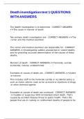
a. Draw a model for length, label it in terms of mu and sigma, and make clear what the
68-95-99.7 rule predicts
Standard numbers!:
- Between plus 1 and minus 1 = 68%
- Between 0 and plus OR minus 1 = 34%
- Between plus 1 and plus 2 OR minus 1 and minus 2 = 13.5%
- Between plus 2 and plus 3 OR minus 2 and minus 3 = 2.5%
- Between plus 1 and plus 3 OR minus 1 and minus 3 = 16%
- Between 0 and plus 3 OR 0 and minus 3 = 50% (49.85)
- Plus 3 standard deviations away from the mean = 1.9949 meters
- Minus 3 standard deviations away from the mean = 1.571 meters
b. Give the interval you would expect for the central 68% in terms of length
→ between 1.697 and 1.823 meter
c. About what percentage of students do you expect to have a length of more than 1.823
meter?
→ 100 – 68 = = 16%
d. About what percentage of students do you expect to have a length between 1.823 and
1.886 meter?
→ 16% - 2.5% = 13.5%
e. What is the length of the shortest 2.5% of students?
→ 1.634 meters or shorter
4
Notes Inferential Statistics – Test 1 ....................................................................................................................... 2
Self-Study B: the normal model + finding probabilities ...................................................................................... 2
Lecture 1: Introduction to statistical inference. Sampling Distribution Model for A PROPORTION and
Confidence intervals for PROPORTIONS........................................................................................................... 8
Statistical inference and the fundamental problem of uncertainty in statistics ............................................... 8
Sampling distribution model FOR PROPORTIONS (theory + assumptions) ................................................... 10
Using the theory about the Sampling Distribution Model for PROPORTIONS (theoretical examples, canvas
page 1.1: ex1 (first year student), ex3 + ex4) .................................................................................................... 13
5. Using the theory about the Sampling Distribution Model for PROPORTIONS in practice: → Confidence
interval for a proportion .................................................................................................................................... 15
1.1: Sampling distribution model for proportions ............................................................................................. 17
Exercises 1.1 Canvas ......................................................................................................................................... 17
1.2: Confidence intervals for proportions .......................................................................................................... 19
Exercises 1.2 Canvas ......................................................................................................................................... 19
Lecture 2: Inference about one mean: Confidence intervals (SDM + CLT + TEST) .................................... 23
Sampling distribution model for a mean............................................................................................................ 23
Inference for means: confidence interval for a mean ........................................................................................ 26
2.1: Sampling distribution model for means (SDM + CLT + TEST) .............................................................. 29
Exercises Canvas ............................................................................................................................................... 29
2.2: Confidence interval for a mean .................................................................................................................... 33
Exercises Canvas ............................................................................................................................................... 35
Reflection Session 1: CI Proportions and Means .............................................................................................. 39
Lecture 3: Inference for means – Test for one mean......................................................................................... 45
Inference for means: hypothesis test for one mean............................................................................................ 45
An example of the one sample t-test................................................................................................................... 48
So an conclusion / overview t-procedure for the one sample situation: ............................................................ 55
Lecture 3B: More about tests .............................................................................................................................. 56
Interpretation of outcomes (statistical significance, magnitude (grootte) of the outcome and practical
significance) ....................................................................................................................................................... 56
Investigating normality: Descriptive + Shapiro-Wilk test................................................................................. 57
More about assumptions and an alternative solution (when to use the Sign test)............................................. 60
Canvas Lecture 3B: more about tests – part II.................................................................................................. 61
1
,3.1: Steps in performing a statistical test ............................................................................................................ 68
3.2: Exercises One-Sample t-test ......................................................................................................................... 69
3.3: Exercises More about Tests .......................................................................................................................... 82
Notes Inferential Statistics – Test 1
Self-Study B: the normal model + finding probabilities
Normal model = N(mu, sigma)
Standard normal model (or: Z-distribution) = N(0,1)
Exercises via the distribution of IQ-scores
Assume: normal distribution
- Mean = 100
- SD = 16
→ IQ has a N(100, 16)-distribution
1. What percentage of observations is expected to fall within one standard deviation
from the mean and what are the borders of that interval?
→ 68% of values fall within 1 SD from the mean
→ 68% of the values fall between: 100 – 16 = 84 & 100 + 16 = 116
2. What percentage of observations is expected to fall within two standard deviations
from the mean and what are the borders of that interval?
→ 95% of values fall within 2 SD from the mean
→ 95% of the values fall between: 100 – 32 = 68 & 100 + 32 = 132
3. What is the expected proportion that has at least a score of 132 or more on the IQ-
scale?
→ IQ-score of 132 is at least 2 SD away from the mean.
→This means that 100 – 95 = 5% / 2 = 2,5% has at least a score of 132 or more.
Using the N(0, 1)-distribution and reading the z-table
Calculating z-scores by:
(observation – mean of population (mu) ) / SD (sigma)
Proportions on Z-table = part below
1 - proportions on Z-table = part above
4. How big is the group with an IQ-score of 124 or more? (What is the expected
proportion that has at least a score of 124 or more on the IQ-scale?)
▪ 4a. What is the standardized score, the z-value, for the IQ-score 124?
→ 124 – 100 (mean) / 16 (SD) = 1.5
▪ 4b. What is the expected proportion that has at least a score of 124 or more on the IQ-
scale? (assuming a normal model)
2
, (use Z-table with Standardized Normal Probabilities)
→ So P(Z > 1.5) = ?
→ In the Z-table you see when Z is 1.5, the SNP is .9332.
→ Expected proportion that has 124+ IQ = 1 – 0.9332 = 0.0668 = 6.68%
Other examples
- What percent of a standard normal model is found for: z < 2.25?
→ .9878 (see Z-table) = 98.78%
- What percent of a standard normal model is found for: -1 < z < 1.15?
→ 1.15 = .8749 & -1 = .1587
→ .8749 - .1587 = .7162 = 71.62%
- Reversing the problem. How can we find the z-value for a certain cumulative
probability?
o What is the value of Z for the highest 75%? →
100 – 75 = 25% = 0,2500.
Z-table says .2514 is closest, so Z-score = -.67
Z-table says there are two values near the probability of .9500, namely .9495 with a Z-
value of 1.64 & .9505 with a Z-value of 1.65. --> We take the z-value in between:
1.645
Specific value for the length
→ z = (y – mu) / sigma
→ 1.645 = (y – 1.76) / .063 = (1.645 * .063) + 1.76 = 1.864 meter
Exercise 1: Temperatures
The high temperature in a town seems to be 2 degrees Celsius on average in January, with a
standard deviation of 6 degrees. In July the mean high temperature is on average 24 degrees
Celsius, with a standard deviation of 5 degrees. In which month is it more unusual to have a
day with a high temperature of 13 degrees?
→ Distance is for both the same, but the probability (normal model) is not the same
o 13 – 2 (= mean January) = 11 & 24 (= mean July) – 13 = 11
→ In January, with mean 2 and SD 6, a high temperature of 13 is almost 2 standard deviations
above the mean ( = 1.83 SD)
→ in July, with mean 24 and SD 5, a high temperature of 13 is more than two standard
deviations below the mean ( = 2.2 SD)
→ So a high temperature of 13 degrees Celsius is less likely to happen in July, when 13
degrees Celsius is farther away from the mean
Exercise 1b: Temperatures
A town’s January high temperatures average 36F with a standard deviation of 10, while in
July the mean high temperature 74 and the standard deviation is 8. In which month is it more
unusual to have a day with a high temperature of 55? Explain.
→ Distance is for both the same, but the probability (normal model) is not the same
o January = 55 – 36 = 19 & distance July = 74 – 55 = 19
3
, → In January, with mean 36 and SD 10, a high temperature of 55 is almost 2 standard
deviations above the mean (19/10 = 1.9 SD)
→ In July, with mean 74 and SD 8, a high temperature of 55 is more than two standard
deviations below the mean (19/8 = 2.375 SD)
→ so a high temperature of 55 is less likely to happen in July, when 55 is farther away from
the mean
Exercise 2: Length of students
- Mean = 1.76 meter
- SD = 0.63 meter
- Assumed we can apply normal model
a. Draw a model for length, label it in terms of mu and sigma, and make clear what the
68-95-99.7 rule predicts
Standard numbers!:
- Between plus 1 and minus 1 = 68%
- Between 0 and plus OR minus 1 = 34%
- Between plus 1 and plus 2 OR minus 1 and minus 2 = 13.5%
- Between plus 2 and plus 3 OR minus 2 and minus 3 = 2.5%
- Between plus 1 and plus 3 OR minus 1 and minus 3 = 16%
- Between 0 and plus 3 OR 0 and minus 3 = 50% (49.85)
- Plus 3 standard deviations away from the mean = 1.9949 meters
- Minus 3 standard deviations away from the mean = 1.571 meters
b. Give the interval you would expect for the central 68% in terms of length
→ between 1.697 and 1.823 meter
c. About what percentage of students do you expect to have a length of more than 1.823
meter?
→ 100 – 68 = = 16%
d. About what percentage of students do you expect to have a length between 1.823 and
1.886 meter?
→ 16% - 2.5% = 13.5%
e. What is the length of the shortest 2.5% of students?
→ 1.634 meters or shorter
4