Lecture 1: Introduction
Machine learning provides systems the ability to automatically learn and improve from
experience without being explicitly programmed. Usually deals with offline learning > train
model once and then it's done. Then use this model.
When to use ML?
• we can’t solve it explicitly. • approximate solutions are fine • plenty of examples available.
(for example: recommendation systems for movies)
ML allows us to learn programs that we have no idea how to write ourselves. Machine
learning allows us to create programs from a set of examples.
Supervised learning (labeled data/have examples)
1. Classification
instances = data example line
features (of the instances) = things we measure (numeric/categorical)
target (value) = what we are trying to learn
Example 1: Linear classifier
loss(model) = performance of model on the data (the lower the better) for classification: e.g.
the number of misclassified examples. used to search the model space. Input: model, has
data as constant.
Example 2: A decision tree classifier = studies one feature in isolation at every node.
Example 3: K-nearest neighbours: lazy: for a new point, it looks at k points that are closest
(k=7 f.e.) and assigns the class that is most frequent in that set. k is what we call a
hyperparameter: you have to choose it yourself before you use the algorithm. Trial &
error/grid search/random search
Variations:
• Features: usually numerical or categorical.
• Binary classification: two classes, usually negative and positive (pos = what you are trying
to detect)
1
,• Multiclass classifcation: more than two classes
• Multilabel classifcation: more than two classes and none, some or all of them may be true
• Class probabilities/scores: the classifer reports a probability for each class.
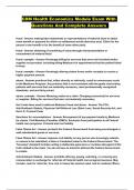
2. Regression
Loss function for regression: the Mean-squared-errors
(MSE) loss → Measure the distance to the line, this is the
difference between what the model predicts and the actual
values of the data. Take all values and square them: so
they are all positive (& so they don’t cancel each other
out). Sum them up, and then divide by size of dataset
(average). the lower MSE, the better (blue line residual)
Assumes normality, so sensitive to outliers
Example 1. Linear regression (straight line)
Example 2. Regression tree (go through every point)
Example 3. kNN regression (take K=x closest points)
Grouping models segment the feature space. Grading models can assign each element in
the feature space a different prediction. Grouping models can only assign a finite number of
predictions.
Grouping model ROC curves have as many line segments as there are instance
space segments in the model; grading models have one line segment for each example
in the data set. This is a concrete manifestation of something I mentioned in the Prologue:
grading models have a much higher ‘resolution’ than grouping models; this is
also called the model’s refinement. by decreasing a model’s refinement we sometimes
achieve better ranking performance.
Overfitting = Our model doesn’t generalize well from our training data to unseen data; it
draws too any specific conclusions from the training data. If our model does much better on
the training set than on the test set, then we’re likely overfitting.
~Split your test and training data!~
Aim of ML is to not to minimize loss on training data, but to minimize on test data.
How to prevent? Never judge our model on how well it does on the training data.We withhold
some data, and test the performance on that. The proportion of test dat you withhold is not
very important. It should be at least 100 instances, although more is better. To avoid
overfitting, the number of parameters estimated from the data must be considerably less
than the number of data points.
Unsupervised learning tasks( unlabeled data)
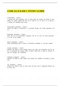
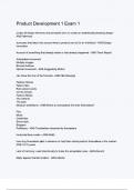
1. Clustering → split the instances into a number of (given)
clusters. Example of clustering algorithm: K-means. In the
example we will separate the dataset shown in (a) into three
clusters. It starts by picking 3 main points, and color them by
the mean color they are close to. Do this again, and throw
away old coloring. Keep doing this until done.
2
,2. Density estimation → when we want to learn how likely new data/examples is. Is a 2 m
tall 16 year old more or less likely than a 1.5 m tall 80 year old? (normal distribution simple
form of density estimation)
3. Generative modelling (sampling)
With complex models, it’s often easier to sample from a probability distribution that it is to get
a density estimate. Sample pictures to get new sample.
Lecture 2: Linear models 1
Optimization= trying to find the input for which a particular function is at its optimum (in this
case its minimum value)
Random search = pick a random point and pick a point quite close to it and see which one
is better. If the new point is better, move to this new point and go again, if new point isn't
better, you discard it. Sensitive to local minimum
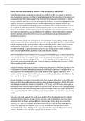
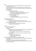
Convex= if you pick any two random points on the loss surface and
draw a line between them, everything in between those points need to
be below that line: practically means that we have 1 (global) minimum
and this minimum is the optimal model. So long as we know we’re
moving down (to a point with lower loss), we can be sure we’re moving
in the direction of the minimum.
What if the loss surface has multiple local minima?
1. Simulated annealing = similar to random search but little difference: if the next point
chosen isn’t better than the current one, we still pick it, but only with some small probability
P. In other words, we allow the algorithm to occasionally travel uphill. This means that
whenever it gets stuck in a local minimum, it still has some probability of escaping, and
finding the global minimum.
→ Random search & simulated annealing: black box optimization (--> don't need to know
specific information/insight/compute gradient about model, only need to compute/evaluate
loss function)
Features: very simple • can require many iterations (takes long, can get stuck in local
minimum) • also works for discrete model spaces
2. Run random search a couple of times independently. One of these runs may start you off
close enough to the global minimum. For simulated annealing, doing multiple runs makes
less sense since it doesn’t get stuck. If you wait long enough, it will find it.
To escape local minima→ add randomness (SA)
To converge (= find certain point) faster → inspect the local neighbourhood (to determine in
which direction the function decreases quickest)
3
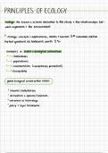
, Gradient descent: start with a random point, we compute the gradient and subtract it from
the current choice ( because the gradient is the direction of steepest descent that we want to
go downhill) and iterate this process. only for continuous models
Since the gradient is only a linear approximation to our loss
function, the bigger our step the bigger the approximation
error. Usually we scale down the step size indicated by the
gradient by multiplying it by a learning rate η. This value is
chosen by trial and error, and remains constant throughout the
search. If our function is non-convex, gradient descent doesn’t
help us with local minima → add a bit of randomness
Sometimes your loss function should not be the same as your
evaluation function.
Loss functions serve two purposes:
1. to express what quality we want to maximise in our search for a good model
2. to provide a smooth loss surface( so that the search for a minimum can be performed
efficiently)
Lecture 3: Methodology 1
Class imbalance= the proportion of the positive class is so small in relation to the negative
class that the accuracy doesn’t mean anything. For example: you create a classification
model and get 90% accuracy immediately, but you discover that 90% of the data belongs to
one class. Do not assume a high accuracy is a good accuracy!
Cost imbalance= the cost of getting it wrong way one way vs the other is very different.
(diagnosing a healthy person with cancer (lower) vs. diagnosing a person with cancer as
healthy (higher)) Both come with a cost but not the same cost (spam vs. ham)
The simplest and most useful sanity check for any machine learning research, is to use
baselines → a simple approach to your problem to
which you compare your results: it helps to calibrate
your expectations for a particular performance
measure on a particular task.
Hyperparameters are the parameters that are
chosen, not learned from the data.
How do we choose the hyper parameter? Ideally, we
try a few and pick the best. However, it would be a
mistake to use the test set for this.
Different tests for accuracy may give different results,
because of too small test data or testing too many
different things on one test set.
4
Machine learning provides systems the ability to automatically learn and improve from
experience without being explicitly programmed. Usually deals with offline learning > train
model once and then it's done. Then use this model.
When to use ML?
• we can’t solve it explicitly. • approximate solutions are fine • plenty of examples available.
(for example: recommendation systems for movies)
ML allows us to learn programs that we have no idea how to write ourselves. Machine
learning allows us to create programs from a set of examples.
Supervised learning (labeled data/have examples)
1. Classification
instances = data example line
features (of the instances) = things we measure (numeric/categorical)
target (value) = what we are trying to learn
Example 1: Linear classifier
loss(model) = performance of model on the data (the lower the better) for classification: e.g.
the number of misclassified examples. used to search the model space. Input: model, has
data as constant.
Example 2: A decision tree classifier = studies one feature in isolation at every node.
Example 3: K-nearest neighbours: lazy: for a new point, it looks at k points that are closest
(k=7 f.e.) and assigns the class that is most frequent in that set. k is what we call a
hyperparameter: you have to choose it yourself before you use the algorithm. Trial &
error/grid search/random search
Variations:
• Features: usually numerical or categorical.
• Binary classification: two classes, usually negative and positive (pos = what you are trying
to detect)
1
,• Multiclass classifcation: more than two classes
• Multilabel classifcation: more than two classes and none, some or all of them may be true
• Class probabilities/scores: the classifer reports a probability for each class.
2. Regression
Loss function for regression: the Mean-squared-errors
(MSE) loss → Measure the distance to the line, this is the
difference between what the model predicts and the actual
values of the data. Take all values and square them: so
they are all positive (& so they don’t cancel each other
out). Sum them up, and then divide by size of dataset
(average). the lower MSE, the better (blue line residual)
Assumes normality, so sensitive to outliers
Example 1. Linear regression (straight line)
Example 2. Regression tree (go through every point)
Example 3. kNN regression (take K=x closest points)
Grouping models segment the feature space. Grading models can assign each element in
the feature space a different prediction. Grouping models can only assign a finite number of
predictions.
Grouping model ROC curves have as many line segments as there are instance
space segments in the model; grading models have one line segment for each example
in the data set. This is a concrete manifestation of something I mentioned in the Prologue:
grading models have a much higher ‘resolution’ than grouping models; this is
also called the model’s refinement. by decreasing a model’s refinement we sometimes
achieve better ranking performance.
Overfitting = Our model doesn’t generalize well from our training data to unseen data; it
draws too any specific conclusions from the training data. If our model does much better on
the training set than on the test set, then we’re likely overfitting.
~Split your test and training data!~
Aim of ML is to not to minimize loss on training data, but to minimize on test data.
How to prevent? Never judge our model on how well it does on the training data.We withhold
some data, and test the performance on that. The proportion of test dat you withhold is not
very important. It should be at least 100 instances, although more is better. To avoid
overfitting, the number of parameters estimated from the data must be considerably less
than the number of data points.
Unsupervised learning tasks( unlabeled data)
1. Clustering → split the instances into a number of (given)
clusters. Example of clustering algorithm: K-means. In the
example we will separate the dataset shown in (a) into three
clusters. It starts by picking 3 main points, and color them by
the mean color they are close to. Do this again, and throw
away old coloring. Keep doing this until done.
2
,2. Density estimation → when we want to learn how likely new data/examples is. Is a 2 m
tall 16 year old more or less likely than a 1.5 m tall 80 year old? (normal distribution simple
form of density estimation)
3. Generative modelling (sampling)
With complex models, it’s often easier to sample from a probability distribution that it is to get
a density estimate. Sample pictures to get new sample.
Lecture 2: Linear models 1
Optimization= trying to find the input for which a particular function is at its optimum (in this
case its minimum value)
Random search = pick a random point and pick a point quite close to it and see which one
is better. If the new point is better, move to this new point and go again, if new point isn't
better, you discard it. Sensitive to local minimum
Convex= if you pick any two random points on the loss surface and
draw a line between them, everything in between those points need to
be below that line: practically means that we have 1 (global) minimum
and this minimum is the optimal model. So long as we know we’re
moving down (to a point with lower loss), we can be sure we’re moving
in the direction of the minimum.
What if the loss surface has multiple local minima?
1. Simulated annealing = similar to random search but little difference: if the next point
chosen isn’t better than the current one, we still pick it, but only with some small probability
P. In other words, we allow the algorithm to occasionally travel uphill. This means that
whenever it gets stuck in a local minimum, it still has some probability of escaping, and
finding the global minimum.
→ Random search & simulated annealing: black box optimization (--> don't need to know
specific information/insight/compute gradient about model, only need to compute/evaluate
loss function)
Features: very simple • can require many iterations (takes long, can get stuck in local
minimum) • also works for discrete model spaces
2. Run random search a couple of times independently. One of these runs may start you off
close enough to the global minimum. For simulated annealing, doing multiple runs makes
less sense since it doesn’t get stuck. If you wait long enough, it will find it.
To escape local minima→ add randomness (SA)
To converge (= find certain point) faster → inspect the local neighbourhood (to determine in
which direction the function decreases quickest)
3
, Gradient descent: start with a random point, we compute the gradient and subtract it from
the current choice ( because the gradient is the direction of steepest descent that we want to
go downhill) and iterate this process. only for continuous models
Since the gradient is only a linear approximation to our loss
function, the bigger our step the bigger the approximation
error. Usually we scale down the step size indicated by the
gradient by multiplying it by a learning rate η. This value is
chosen by trial and error, and remains constant throughout the
search. If our function is non-convex, gradient descent doesn’t
help us with local minima → add a bit of randomness
Sometimes your loss function should not be the same as your
evaluation function.
Loss functions serve two purposes:
1. to express what quality we want to maximise in our search for a good model
2. to provide a smooth loss surface( so that the search for a minimum can be performed
efficiently)
Lecture 3: Methodology 1
Class imbalance= the proportion of the positive class is so small in relation to the negative
class that the accuracy doesn’t mean anything. For example: you create a classification
model and get 90% accuracy immediately, but you discover that 90% of the data belongs to
one class. Do not assume a high accuracy is a good accuracy!
Cost imbalance= the cost of getting it wrong way one way vs the other is very different.
(diagnosing a healthy person with cancer (lower) vs. diagnosing a person with cancer as
healthy (higher)) Both come with a cost but not the same cost (spam vs. ham)
The simplest and most useful sanity check for any machine learning research, is to use
baselines → a simple approach to your problem to
which you compare your results: it helps to calibrate
your expectations for a particular performance
measure on a particular task.
Hyperparameters are the parameters that are
chosen, not learned from the data.
How do we choose the hyper parameter? Ideally, we
try a few and pick the best. However, it would be a
mistake to use the test set for this.
Different tests for accuracy may give different results,
because of too small test data or testing too many
different things on one test set.
4