PSY4107 –
Advanced
Statistics II
RMA Cognitive and Clinical Science Period 3
(Maastricht University)
This course focuses on repeated measures designs and starts with a review of oneway and
twoway within-subject designs, and split-plot designs with a covariate. This review is
followed by a treatment of mixed (multilevel) linear regression for nested and longitudinal
designs. We will start this treatment with so-called marginal models for repeated measures
as a flexible alternative to repeated measures ANOVA in case of missing data or within-
subject covariates, and end with random effects models for repeated measures and nested
designs. Part II concludes with the topic of optimal design and sample size.
This is a personal summary of this course. Therefore, this summary may contain errors and does
not replace the knowledge a student should acquire throughout this course.
February 2017
, Table of Content
Topic 1 - Oneway within-subject ANOVA ............................................................................................. 3
Lecture 1 .............................................................................................................................................. 3
Practical Lecture 1 ............................................................................................................................. 13
Meeting 1........................................................................................................................................... 20
2010 ............................................................................................................................................... 20
2011 ............................................................................................................................................... 21
2012 ............................................................................................................................................... 22
Topic 2 - Twoway WS ANOVA and split-plot (BS*WS) ANOVA ..................................................... 24
Lecture 2 ............................................................................................................................................ 24
Practical Lecture 2 ............................................................................................................................. 38
Meeting 2........................................................................................................................................... 47
2010 ............................................................................................................................................... 47
2011 ............................................................................................................................................... 49
2012 ............................................................................................................................................... 51
Topic 3 - Covariates in WS and split-plot ANOVA.............................................................................. 55
Lecture 3 ............................................................................................................................................ 55
Practical Lecture 3 ............................................................................................................................. 67
Meeting 3........................................................................................................................................... 75
2010 ............................................................................................................................................... 75
2011 ............................................................................................................................................... 76
2012 ............................................................................................................................................... 78
Topic 4 - Mixed (multilevel) regression for longitudinal data: marginal models ................................. 79
Lecture 4 ............................................................................................................................................ 79
Practical Lecture 4 ............................................................................................................................. 92
Meeting 4......................................................................................................................................... 101
2010 ............................................................................................................................................. 101
2011 ............................................................................................................................................. 104
Topic 5 - Mixed regression for longitudinal and nested data: random intercept ................................. 106
Lecture 5 .......................................................................................................................................... 106
Practical Lecture 5 ........................................................................................................................... 121
Meeting 5......................................................................................................................................... 129
2010 ............................................................................................................................................. 129
2011 ............................................................................................................................................. 130
Topic 6 - Mixed regression for longitudinal and nested data: random slope ...................................... 133
Lecture 6 .......................................................................................................................................... 133
1
, Practical Lecture 6 ........................................................................................................................... 146
Meeting 6......................................................................................................................................... 158
2012 ............................................................................................................................................. 158
Topic 7 - Optimal design, sample size ................................................................................................ 163
Lecture 7 .......................................................................................................................................... 163
Practical Lecture 7 ........................................................................................................................... 175
Meeting 7......................................................................................................................................... 181
2010 ............................................................................................................................................. 181
2011 ............................................................................................................................................. 182
2012 ............................................................................................................................................. 183
Task Notes ........................................................................................................................................... 185
Appendix: Chi square values ............................................................................................................... 191
2
,Topic 1 - Oneway within-subject ANOVA
Lecture 1
What is a WS design?
o K repeated measures of a (quantitative) outcome Y
o On the same N persons (or animals, families etc.)
o under K conditions or at K time points
Types of WS design
o WS exp, replications blocked, crossover
N = 40 students
K= 4 conditions (stand, rest, bonus, rest+bonus)
192 trials per conditions, presented in blocked order
condition order counterbalanced BS (Latin square)
outcome: mean RT
(per set of 6 trials, 32 sets per person per condition)
o WS exp, replications mixed, event-related design
N = 12 students
K = 4 angles of rotation (x same/different)
32 trials per angle (16 same, 16 diff), mixed
outcome: mean RT of all 32 trials
(per person per angle)
3
, o observational studies: growth curves (VGT – Progress test)
o repeated measures in BS exp (BS*WS = split-plot)
Within-subject versus between-subject:
o Advantages and drawbacks
Advantages:
much smaller N of persons needed
each person is his/her own control
Drawbacks:
not feasible in case of irreversible treatment effect
risk of „carry over„ effects (wash-out needed)
o Sample size
For comparing two conditions on a quantitative Y:
BS: unpaired t-test (or 1-way BS ANOVA)
WS: paired t-test (or 1-way WS ANOVA)
Due to smaller residual outcome variance, and observing
each subject in each condition, WS needs only (1-ρ)/2 × total
sample size of BS, where ρ = correlation between paired
samples
o Reduced SS(error)
4
, Univariate method
o The model
o Estimation
If only 1 observation: you cannot separate interaction
Interaction effect = (Yij –Yi – Yj + Ytotal)
With only 1 observation interaction effect and residual is same
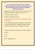
o Example: raw data
o Example: SS(total)
Sum of squares
(-3)2 + (-1)2 = 10
Individual score (Yij) – Grand mean (Y)
6 – 10 = -4
5
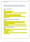
,o Example: SS(condition)
Condition mean (Yj) – Grand mean (Y)
8 – 10 = -2
o Example: SS (person)
Person mean (Yi) – Grand mean (Y)
8 – 10 = -2
o Example: SS(residual)
Individual score (Yij) – Person/ Condition marginal mean
7–8=1
o Testing
Dividing by df gives the MS‟s for F-test, but:
Only 1 observation per cell (= person x condition
→ Interaction + error cannot be separated, MS(residual) is a
mix of interaction and error!
And person is random, not fixed → affects E(MS)
So what is the corrected F-test then?
6
, o Denominator of F
1-way WS design: treat fixed, person random, so:
if > 1 repli: test treat effect against interaction
if = 1 repli: test treat effect against residual (error+interaction pooled)
then: person and person*treat effects untestable. But who
wants to test these anyway?
(There would only be one time point at which person is tested
and to differentiate person effect and person*treatment effect
you would need at least 2 different time points)
→“You don’t have to understand the details, just believe it”
choice of denominator of F follows from the E(MS) table for that design
ANOVA of raw RTs ( > 1 replications per cell) gives the same F and p for the
condition effect as does ANOVA of average RT across trials !
in example: F= MS(cond) / MS(resid) = .67
o Sphericity
assumption: sphericity
= each pairwise difference has same variance
→ each pairwise comparison same SE (= SD / √n)
≈ compound symmetry: same variance in each condition, same
correlation in all pairs of conditions
Problem: Rarely valid if K > 2 conditions
larger type I error risk for F-test
too small / too large SE‟s for pairwise comparisons (higher risk of TI
errors for some and TII for others)
Solutions:
Epsilon-adjustment of df in univariate ANOVA:
o Multiply df(numerator) and df(denominator) with a factor
epsilon (ε) < 1
→ critical F-value higher
lower-bound ε = 1/(K-1) , is an overcorrection
(overcorrection more extreme with more conditions)
Better: GG (or HF) , ε lower (critical F higher) as
sphericity is more strongly violated.
“You do not have to know how it is computed”
multivariate ANOVA
From SUMMARY OF LECTURE
7
Advanced
Statistics II
RMA Cognitive and Clinical Science Period 3
(Maastricht University)
This course focuses on repeated measures designs and starts with a review of oneway and
twoway within-subject designs, and split-plot designs with a covariate. This review is
followed by a treatment of mixed (multilevel) linear regression for nested and longitudinal
designs. We will start this treatment with so-called marginal models for repeated measures
as a flexible alternative to repeated measures ANOVA in case of missing data or within-
subject covariates, and end with random effects models for repeated measures and nested
designs. Part II concludes with the topic of optimal design and sample size.
This is a personal summary of this course. Therefore, this summary may contain errors and does
not replace the knowledge a student should acquire throughout this course.
February 2017
, Table of Content
Topic 1 - Oneway within-subject ANOVA ............................................................................................. 3
Lecture 1 .............................................................................................................................................. 3
Practical Lecture 1 ............................................................................................................................. 13
Meeting 1........................................................................................................................................... 20
2010 ............................................................................................................................................... 20
2011 ............................................................................................................................................... 21
2012 ............................................................................................................................................... 22
Topic 2 - Twoway WS ANOVA and split-plot (BS*WS) ANOVA ..................................................... 24
Lecture 2 ............................................................................................................................................ 24
Practical Lecture 2 ............................................................................................................................. 38
Meeting 2........................................................................................................................................... 47
2010 ............................................................................................................................................... 47
2011 ............................................................................................................................................... 49
2012 ............................................................................................................................................... 51
Topic 3 - Covariates in WS and split-plot ANOVA.............................................................................. 55
Lecture 3 ............................................................................................................................................ 55
Practical Lecture 3 ............................................................................................................................. 67
Meeting 3........................................................................................................................................... 75
2010 ............................................................................................................................................... 75
2011 ............................................................................................................................................... 76
2012 ............................................................................................................................................... 78
Topic 4 - Mixed (multilevel) regression for longitudinal data: marginal models ................................. 79
Lecture 4 ............................................................................................................................................ 79
Practical Lecture 4 ............................................................................................................................. 92
Meeting 4......................................................................................................................................... 101
2010 ............................................................................................................................................. 101
2011 ............................................................................................................................................. 104
Topic 5 - Mixed regression for longitudinal and nested data: random intercept ................................. 106
Lecture 5 .......................................................................................................................................... 106
Practical Lecture 5 ........................................................................................................................... 121
Meeting 5......................................................................................................................................... 129
2010 ............................................................................................................................................. 129
2011 ............................................................................................................................................. 130
Topic 6 - Mixed regression for longitudinal and nested data: random slope ...................................... 133
Lecture 6 .......................................................................................................................................... 133
1
, Practical Lecture 6 ........................................................................................................................... 146
Meeting 6......................................................................................................................................... 158
2012 ............................................................................................................................................. 158
Topic 7 - Optimal design, sample size ................................................................................................ 163
Lecture 7 .......................................................................................................................................... 163
Practical Lecture 7 ........................................................................................................................... 175
Meeting 7......................................................................................................................................... 181
2010 ............................................................................................................................................. 181
2011 ............................................................................................................................................. 182
2012 ............................................................................................................................................. 183
Task Notes ........................................................................................................................................... 185
Appendix: Chi square values ............................................................................................................... 191
2
,Topic 1 - Oneway within-subject ANOVA
Lecture 1
What is a WS design?
o K repeated measures of a (quantitative) outcome Y
o On the same N persons (or animals, families etc.)
o under K conditions or at K time points
Types of WS design
o WS exp, replications blocked, crossover
N = 40 students
K= 4 conditions (stand, rest, bonus, rest+bonus)
192 trials per conditions, presented in blocked order
condition order counterbalanced BS (Latin square)
outcome: mean RT
(per set of 6 trials, 32 sets per person per condition)
o WS exp, replications mixed, event-related design
N = 12 students
K = 4 angles of rotation (x same/different)
32 trials per angle (16 same, 16 diff), mixed
outcome: mean RT of all 32 trials
(per person per angle)
3
, o observational studies: growth curves (VGT – Progress test)
o repeated measures in BS exp (BS*WS = split-plot)
Within-subject versus between-subject:
o Advantages and drawbacks
Advantages:
much smaller N of persons needed
each person is his/her own control
Drawbacks:
not feasible in case of irreversible treatment effect
risk of „carry over„ effects (wash-out needed)
o Sample size
For comparing two conditions on a quantitative Y:
BS: unpaired t-test (or 1-way BS ANOVA)
WS: paired t-test (or 1-way WS ANOVA)
Due to smaller residual outcome variance, and observing
each subject in each condition, WS needs only (1-ρ)/2 × total
sample size of BS, where ρ = correlation between paired
samples
o Reduced SS(error)
4
, Univariate method
o The model
o Estimation
If only 1 observation: you cannot separate interaction
Interaction effect = (Yij –Yi – Yj + Ytotal)
With only 1 observation interaction effect and residual is same
o Example: raw data
o Example: SS(total)
Sum of squares
(-3)2 + (-1)2 = 10
Individual score (Yij) – Grand mean (Y)
6 – 10 = -4
5
,o Example: SS(condition)
Condition mean (Yj) – Grand mean (Y)
8 – 10 = -2
o Example: SS (person)
Person mean (Yi) – Grand mean (Y)
8 – 10 = -2
o Example: SS(residual)
Individual score (Yij) – Person/ Condition marginal mean
7–8=1
o Testing
Dividing by df gives the MS‟s for F-test, but:
Only 1 observation per cell (= person x condition
→ Interaction + error cannot be separated, MS(residual) is a
mix of interaction and error!
And person is random, not fixed → affects E(MS)
So what is the corrected F-test then?
6
, o Denominator of F
1-way WS design: treat fixed, person random, so:
if > 1 repli: test treat effect against interaction
if = 1 repli: test treat effect against residual (error+interaction pooled)
then: person and person*treat effects untestable. But who
wants to test these anyway?
(There would only be one time point at which person is tested
and to differentiate person effect and person*treatment effect
you would need at least 2 different time points)
→“You don’t have to understand the details, just believe it”
choice of denominator of F follows from the E(MS) table for that design
ANOVA of raw RTs ( > 1 replications per cell) gives the same F and p for the
condition effect as does ANOVA of average RT across trials !
in example: F= MS(cond) / MS(resid) = .67
o Sphericity
assumption: sphericity
= each pairwise difference has same variance
→ each pairwise comparison same SE (= SD / √n)
≈ compound symmetry: same variance in each condition, same
correlation in all pairs of conditions
Problem: Rarely valid if K > 2 conditions
larger type I error risk for F-test
too small / too large SE‟s for pairwise comparisons (higher risk of TI
errors for some and TII for others)
Solutions:
Epsilon-adjustment of df in univariate ANOVA:
o Multiply df(numerator) and df(denominator) with a factor
epsilon (ε) < 1
→ critical F-value higher
lower-bound ε = 1/(K-1) , is an overcorrection
(overcorrection more extreme with more conditions)
Better: GG (or HF) , ε lower (critical F higher) as
sphericity is more strongly violated.
“You do not have to know how it is computed”
multivariate ANOVA
From SUMMARY OF LECTURE
7