, PROBLEM 1.1
KNOWN: Thermal conductivity, thickness and temperature difference across a sheet of rigid
extruded insulation.
FIND: (a) The heat flux through a 2 m × 2 m sheet of the insulation, and (b) The heat rate
through the sheet.
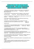
SCHEMATIC:
A = 4 m2
W
k = 0.029
m ⋅K qcond
T1 – T2 = 10˚C
T1 T2
L = 20 mm
x
ASSUMPTIONS: (1) One-dimensional conduction in the x-direction, (2) Steady-state
conditions, (3) Constant properties.
ANALYSIS: From Equation 1.2 the heat flux is
dT T -T
q′′x = -k =k 1 2
dx L
Solving,
W 10 K
q"x = 0.029 ×
m⋅K 0.02 m
W
q′′x = 14.5 <
m2
The heat rate is
W
q x = q′′x ⋅ A = 14.5 2
× 4 m 2 = 58 W <
m
COMMENTS: (1) Be sure to keep in mind the important distinction between the heat flux
(W/m2) and the heat rate (W). (2) The direction of heat flow is from hot to cold. (3) Note that
a temperature difference may be expressed in kelvins or degrees Celsius.
, PROBLEM 1.2
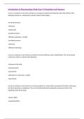
KNOWN: Thickness and thermal conductivity of a wall. Heat flux applied to one face and
temperatures of both surfaces.
FIND: Whether steady-state conditions exist.
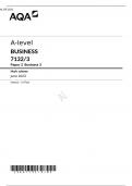
SCHEMATIC:
L = 10 mm
T2 = 30°C
q” = 20 W/m2
q″cond
T1 = 50°C k = 12 W/m·K
ASSUMPTIONS: (1) One-dimensional conduction, (2) Constant properties, (3) No internal energy
generation.
ANALYSIS: Under steady-state conditions an energy balance on the control volume shown is
′′ = qout
qin ′′ = qcond
′′ = k (T1 − T2 ) / L = 12 W/m ⋅ K(50°C − 30°C) / 0.01 m = 24,000 W/m 2
Since the heat flux in at the left face is only 20 W/m2, the conditions are not steady state. <
COMMENTS: If the same heat flux is maintained until steady-state conditions are reached, the
steady-state temperature difference across the wall will be
ΔT = q′′L / k = 20 W/m 2 × 0.01 m /12 W/m ⋅ K = 0.0167 K
which is much smaller than the specified temperature difference of 20°C.
, PROBLEM 1.3
KNOWN: Inner surface temperature and thermal conductivity of a concrete wall.
FIND: Heat loss by conduction through the wall as a function of outer surface temperatures ranging from
-15 to 38°C.
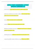
SCHEMATIC:
ASSUMPTIONS: (1) One-dimensional conduction in the x-direction, (2) Steady-state conditions, (3)
Constant properties.
ANALYSIS: From Fourier’s law, if q′′x and k are each constant it is evident that the gradient,
dT dx = − q′′x k , is a constant, and hence the temperature distribution is linear. The heat flux must be
constant under one-dimensional, steady-state conditions; and k is approximately constant if it depends
only weakly on temperature. The heat flux and heat rate when the outside wall temperature is T2 = -15°C
are
q′′x = − k
dT
=k
T1 − T2
= 1W m ⋅ K
25o C − −15o C
= 133.3 W m 2 .
( )
(1)
dx L 0.30 m
q x = q′′x × A = 133.3 W m 2 × 20 m 2 = 2667 W . (2) <
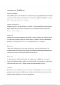
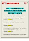
Combining Eqs. (1) and (2), the heat rate qx can be determined for the range of outer surface temperature,
-15 ≤ T2 ≤ 38°C, with different wall thermal conductivities, k.
3500
2500
Heat loss, qx (W)
1500
500
-500
-1500
-20 -10 0 10 20 30 40
Ambient
Outside air temperature, T2 (C)
surface
Wall thermal conductivity, k = 1.25 W/m.K
k = 1 W/m.K, concrete wall
k = 0.75 W/m.K
For the concrete wall, k = 1 W/m⋅K, the heat loss varies linearly from +2667 W to -867 W and is zero
when the inside and outer surface temperatures are the same. The magnitude of the heat rate increases
with increasing thermal conductivity.
COMMENTS: Without steady-state conditions and constant k, the temperature distribution in a plane
wall would not be linear.
KNOWN: Thermal conductivity, thickness and temperature difference across a sheet of rigid
extruded insulation.
FIND: (a) The heat flux through a 2 m × 2 m sheet of the insulation, and (b) The heat rate
through the sheet.
SCHEMATIC:
A = 4 m2
W
k = 0.029
m ⋅K qcond
T1 – T2 = 10˚C
T1 T2
L = 20 mm
x
ASSUMPTIONS: (1) One-dimensional conduction in the x-direction, (2) Steady-state
conditions, (3) Constant properties.
ANALYSIS: From Equation 1.2 the heat flux is
dT T -T
q′′x = -k =k 1 2
dx L
Solving,
W 10 K
q"x = 0.029 ×
m⋅K 0.02 m
W
q′′x = 14.5 <
m2
The heat rate is
W
q x = q′′x ⋅ A = 14.5 2
× 4 m 2 = 58 W <
m
COMMENTS: (1) Be sure to keep in mind the important distinction between the heat flux
(W/m2) and the heat rate (W). (2) The direction of heat flow is from hot to cold. (3) Note that
a temperature difference may be expressed in kelvins or degrees Celsius.
, PROBLEM 1.2
KNOWN: Thickness and thermal conductivity of a wall. Heat flux applied to one face and
temperatures of both surfaces.
FIND: Whether steady-state conditions exist.
SCHEMATIC:
L = 10 mm
T2 = 30°C
q” = 20 W/m2
q″cond
T1 = 50°C k = 12 W/m·K
ASSUMPTIONS: (1) One-dimensional conduction, (2) Constant properties, (3) No internal energy
generation.
ANALYSIS: Under steady-state conditions an energy balance on the control volume shown is
′′ = qout
qin ′′ = qcond
′′ = k (T1 − T2 ) / L = 12 W/m ⋅ K(50°C − 30°C) / 0.01 m = 24,000 W/m 2
Since the heat flux in at the left face is only 20 W/m2, the conditions are not steady state. <
COMMENTS: If the same heat flux is maintained until steady-state conditions are reached, the
steady-state temperature difference across the wall will be
ΔT = q′′L / k = 20 W/m 2 × 0.01 m /12 W/m ⋅ K = 0.0167 K
which is much smaller than the specified temperature difference of 20°C.
, PROBLEM 1.3
KNOWN: Inner surface temperature and thermal conductivity of a concrete wall.
FIND: Heat loss by conduction through the wall as a function of outer surface temperatures ranging from
-15 to 38°C.
SCHEMATIC:
ASSUMPTIONS: (1) One-dimensional conduction in the x-direction, (2) Steady-state conditions, (3)
Constant properties.
ANALYSIS: From Fourier’s law, if q′′x and k are each constant it is evident that the gradient,
dT dx = − q′′x k , is a constant, and hence the temperature distribution is linear. The heat flux must be
constant under one-dimensional, steady-state conditions; and k is approximately constant if it depends
only weakly on temperature. The heat flux and heat rate when the outside wall temperature is T2 = -15°C
are
q′′x = − k
dT
=k
T1 − T2
= 1W m ⋅ K
25o C − −15o C
= 133.3 W m 2 .
( )
(1)
dx L 0.30 m
q x = q′′x × A = 133.3 W m 2 × 20 m 2 = 2667 W . (2) <
Combining Eqs. (1) and (2), the heat rate qx can be determined for the range of outer surface temperature,
-15 ≤ T2 ≤ 38°C, with different wall thermal conductivities, k.
3500
2500
Heat loss, qx (W)
1500
500
-500
-1500
-20 -10 0 10 20 30 40
Ambient
Outside air temperature, T2 (C)
surface
Wall thermal conductivity, k = 1.25 W/m.K
k = 1 W/m.K, concrete wall
k = 0.75 W/m.K
For the concrete wall, k = 1 W/m⋅K, the heat loss varies linearly from +2667 W to -867 W and is zero
when the inside and outer surface temperatures are the same. The magnitude of the heat rate increases
with increasing thermal conductivity.
COMMENTS: Without steady-state conditions and constant k, the temperature distribution in a plane
wall would not be linear.