Fundamentals of Biostatistics 8th Edition Rosner
Solutions Manual
Contents
Chapter 2 Descriptive Statistics........................................................................................................2
Chapter 3 Probability...................................................................................................................... 21
Chapter 4 Discrete Probability Distributions.................................................................................. 43
Chapter 5 Continuous Probability Distributions ............................................................................ 65
Chapter 6 Estimation ...................................................................................................................... 93
Chapter 7 Hypothesis Testing: One-Sample Inference ............................................................... 119
Chapter 8 Hypothesis Testing: Two-Sample Inference ............................................................... 146
Chapter 9 Nonparametric Methods .............................................................................................. 192
Chapter 10 Hypothesis Testing: Categorical Data ....................................................................... 216
Chapter 11 Regression and Correlation Methods ......................................................................... 267
Chapter 12 Multisample Inference ............................................................................................... 322
Chapter 13 Design and Analysis Techniques for Epidemiologic Studies ....................................358
Chapter 14 Hypothesis Testing: Person-Time Data ....................................................................413
, DESCRIPTIVE
STATISTICS
20.1 We have
x=
xi = 215 = 8.6 days
n 25
(n + 1)
median = th largest observation = 13th largest observation = 8 days
2
20.2 We have that
25
(x − x)
2
i
( 5 − 8.6)2 + + ( 4 − 8.6)2 =
784
= 32.67
s2 = i=1 =
24 24 24
s = standard deviation = variance = 5.72 days
range = largest − smallest observation = 30 − 3 = 27 days
20.3 Suppose we divide the patients according to whether or not they received antibiotics, and calculate the
mean and standard deviation for each of the two subsamples:
x s n
Antibiotics 11.57 8.81 7
No antibiotics 7.44 3.70 18
Antibiotics - x7 8.50 3.73 6
It appears that antibiotic users stay longer in the hospital. Note that when we remove observation 7, the
two standard deviations are in substantial agreement, and the difference in the means is not that
impressive anymore. This example shows that x and s2 are not robust; that is, their values are easily
affected by outliers, particularly in small samples. Therefore, we would not conclude that hospital stay is
different for antibiotic users vs. non-antibiotic users.
2
,CHAPTER 2/DESCRIPTIVE STATISTICS 3
2.4-2.7 Changing the scale by a factor c will multiply each data value xi by c, changing it to cxi . Again the same
individual’s value will be at the median and the same individual’s value will be at the mode, but these
values will be multiplied by c. The geometric mean will be multiplied by c also, as can easily be shown:
Geometric mean = [(cx1)(cx2 ) (cxn )]1/n
= (cn x1 x2 xn )1/n
= c( x1 x2 xn )1/n
= c old geometric mean
The range will also be multiplied by c.
For example, if c = 2 we have:
xi
Original Scale
–3 –2 –1 0 1 2 3
xi
Scale 2
–6 –4 –2 0 2 4 6
2.8 We first read the data file “running time” in R
> require(xlsx)
> running<-na.omit(read.xlsx("C:/Data_sets/running_time.xlsx",1,
header=TRUE))
Let us print the first observations
> head(running)
week time
1 1 12.80
2 2 12.20
3 3 12.25
4 4 12.18
5 5 11.53
6 6 12.47
The mean 1-mile running time over 18 weeks is equal to 12.09 minutes:
> mean(running$time)
[1] 12.08889
2.9 The standard deviation is given by
> sd(running$time)
[1] 0.3874181
2.10 Let us first create the variable “time_100” and then calculate its mean and standard deviation
> running$time_100=100*running$time
> mean(running$time_100)
[1] 1208.889
> sd(running$time_100)
[1] 38.74181
2.11 Let us to construct the stem-and-leaf plot in R using the stem.leaf command from the package “aplpack”
> require(aplpack)
, CHAPTER 2/DESCRIPTIVE STATISTICS 4
> stem.leaf(running$time_100, unit=1, trim.outliers=FALSE)
1 | 2: represents 12
leaf unit: 1
n: 18
2 115 | 37
3 116 | 7
5 117 | 23
7 118 | 03
8 119 | 2
(1) 120 | 8
9 121 | 8
8 122 | 05
6 123 | 03
4 124 | 7
3 125 | 5
2 126 | 7
127 |
1 128 | 0
Note: one can also use the standard command stem (which does require the “aplpack” package) to get a similar plot
> stem(running$time_100, scale = 4)
Box plot of running times
2.12 The quantiles of the running times are
12.8
> quantile(running$time) 12.6
0% 25% 50% 75% 100%
11.5300 11.7475 12.1300 12.3225 12.8000 12.4
An outlying value is identify has any value x such that
x upper quartile+1.5 (upper quartile-lower quartile)
Time
12.2
= 12.32 +1.5 (12.32 −11.75) 12.0
= 12.32 + 0.85 = 13.17
11.8
Since 12.97 minutes is smaller than the largest nonoutlying value
(13.17 minutes), this running time recorded in his first week of 11.6
running in the spring is not an outlying value relative to the
distribution of running times recorded the previous year.
2.13 The mean is
x=
xi = 469 = 19.54 mg dL
24 24
2.14 We have that
24
(x − x )
i
2
(49 −19.54)2 + + (12 −19.54)
2
6495.96
s2 = i=1
= = = 282.43
23 23 23
s = 282.43 = 16.81 mg/dL
2.15 We provide two rows for each stem corresponding to leaves 5-9 and 0-4 respectively. We have
Solutions Manual
Contents
Chapter 2 Descriptive Statistics........................................................................................................2
Chapter 3 Probability...................................................................................................................... 21
Chapter 4 Discrete Probability Distributions.................................................................................. 43
Chapter 5 Continuous Probability Distributions ............................................................................ 65
Chapter 6 Estimation ...................................................................................................................... 93
Chapter 7 Hypothesis Testing: One-Sample Inference ............................................................... 119
Chapter 8 Hypothesis Testing: Two-Sample Inference ............................................................... 146
Chapter 9 Nonparametric Methods .............................................................................................. 192
Chapter 10 Hypothesis Testing: Categorical Data ....................................................................... 216
Chapter 11 Regression and Correlation Methods ......................................................................... 267
Chapter 12 Multisample Inference ............................................................................................... 322
Chapter 13 Design and Analysis Techniques for Epidemiologic Studies ....................................358
Chapter 14 Hypothesis Testing: Person-Time Data ....................................................................413
, DESCRIPTIVE
STATISTICS
20.1 We have
x=
xi = 215 = 8.6 days
n 25
(n + 1)
median = th largest observation = 13th largest observation = 8 days
2
20.2 We have that
25
(x − x)
2
i
( 5 − 8.6)2 + + ( 4 − 8.6)2 =
784
= 32.67
s2 = i=1 =
24 24 24
s = standard deviation = variance = 5.72 days
range = largest − smallest observation = 30 − 3 = 27 days
20.3 Suppose we divide the patients according to whether or not they received antibiotics, and calculate the
mean and standard deviation for each of the two subsamples:
x s n
Antibiotics 11.57 8.81 7
No antibiotics 7.44 3.70 18
Antibiotics - x7 8.50 3.73 6
It appears that antibiotic users stay longer in the hospital. Note that when we remove observation 7, the
two standard deviations are in substantial agreement, and the difference in the means is not that
impressive anymore. This example shows that x and s2 are not robust; that is, their values are easily
affected by outliers, particularly in small samples. Therefore, we would not conclude that hospital stay is
different for antibiotic users vs. non-antibiotic users.
2
,CHAPTER 2/DESCRIPTIVE STATISTICS 3
2.4-2.7 Changing the scale by a factor c will multiply each data value xi by c, changing it to cxi . Again the same
individual’s value will be at the median and the same individual’s value will be at the mode, but these
values will be multiplied by c. The geometric mean will be multiplied by c also, as can easily be shown:
Geometric mean = [(cx1)(cx2 ) (cxn )]1/n
= (cn x1 x2 xn )1/n
= c( x1 x2 xn )1/n
= c old geometric mean
The range will also be multiplied by c.
For example, if c = 2 we have:
xi
Original Scale
–3 –2 –1 0 1 2 3
xi
Scale 2
–6 –4 –2 0 2 4 6
2.8 We first read the data file “running time” in R
> require(xlsx)
> running<-na.omit(read.xlsx("C:/Data_sets/running_time.xlsx",1,
header=TRUE))
Let us print the first observations
> head(running)
week time
1 1 12.80
2 2 12.20
3 3 12.25
4 4 12.18
5 5 11.53
6 6 12.47
The mean 1-mile running time over 18 weeks is equal to 12.09 minutes:
> mean(running$time)
[1] 12.08889
2.9 The standard deviation is given by
> sd(running$time)
[1] 0.3874181
2.10 Let us first create the variable “time_100” and then calculate its mean and standard deviation
> running$time_100=100*running$time
> mean(running$time_100)
[1] 1208.889
> sd(running$time_100)
[1] 38.74181
2.11 Let us to construct the stem-and-leaf plot in R using the stem.leaf command from the package “aplpack”
> require(aplpack)
, CHAPTER 2/DESCRIPTIVE STATISTICS 4
> stem.leaf(running$time_100, unit=1, trim.outliers=FALSE)
1 | 2: represents 12
leaf unit: 1
n: 18
2 115 | 37
3 116 | 7
5 117 | 23
7 118 | 03
8 119 | 2
(1) 120 | 8
9 121 | 8
8 122 | 05
6 123 | 03
4 124 | 7
3 125 | 5
2 126 | 7
127 |
1 128 | 0
Note: one can also use the standard command stem (which does require the “aplpack” package) to get a similar plot
> stem(running$time_100, scale = 4)
Box plot of running times
2.12 The quantiles of the running times are
12.8
> quantile(running$time) 12.6
0% 25% 50% 75% 100%
11.5300 11.7475 12.1300 12.3225 12.8000 12.4
An outlying value is identify has any value x such that
x upper quartile+1.5 (upper quartile-lower quartile)
Time
12.2
= 12.32 +1.5 (12.32 −11.75) 12.0
= 12.32 + 0.85 = 13.17
11.8
Since 12.97 minutes is smaller than the largest nonoutlying value
(13.17 minutes), this running time recorded in his first week of 11.6
running in the spring is not an outlying value relative to the
distribution of running times recorded the previous year.
2.13 The mean is
x=
xi = 469 = 19.54 mg dL
24 24
2.14 We have that
24
(x − x )
i
2
(49 −19.54)2 + + (12 −19.54)
2
6495.96
s2 = i=1
= = = 282.43
23 23 23
s = 282.43 = 16.81 mg/dL
2.15 We provide two rows for each stem corresponding to leaves 5-9 and 0-4 respectively. We have