Week 5:
Preparation: Chap 11: Aggregate Demand I: Building the
IS-LM Model
IS-LM model: Model of aggregate demand, leading interpretation of Keynes’
theory.
IS curve: Investment; “investment” and “saving” (market for goods and services)
LM curve: Saving; “liquidity” and “money” (supply and demand for money)
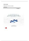
The IS curve plot is the relationship between the interest rate and the level of
income that arises in the market for goods and services.
The Keynesian cross: simplest interpretation of Keynes’s theory of how national
income is determined and is a building block for IS-LM Model.
Actual expenditure: amount households, firms and gov spend on goods and
services = GDP
Planned expenditure: amount the previous would like to spend on goods and
services.
PE = C + I + G
PE = C (Y – T) + I + G
Assumption: The economy is in equilibrium when actual expenditure = planned
expenditure.
So Y = PE
∆Y/∆G is the government-purchases multiplier.
When a government purchase raises income, it raises consumption as well.
∆Y/∆G = 1/(1 – MPC)
∆Y/∆T = - MPC / (1 – MPC) = Tax Multiplier
I = I(r)
The IS curve shows the combinations of the interest rate and the level of
income that are consistent with equilibrium in the market for goods and
services. The IS curve is drawn for a given fiscal policy. Changes in fiscal
policy that raise the demand for goods and services shift the IS curve to
the right. Changes in fiscal policy that reduce the demand for goods and
services shift the IS curve to the left.
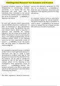
Theory of liquidity preference: a theory of the interest rate.
(M/P)S = M/ P
(M/P)d= L(r)
(M/P)d= L(r, Y)
The LM curve shows the combinations of the interest rate and the level of
income that are consistent with equilibrium in the market for real money
balances. The LM curve is drawn for a given supply of real money
balances. Decreases in the supply of real money balances shift the LM
curve upward. Increases in the supply of real money balances shift the LM
curve downward.
, Chap 12: Aggregate Demand II: Applying the IS-
LM Model
Monetary transmission mechanism: how a monetary expansion induces greater
spending on goods and services.
IS-LM model shows that an increase in the money supply lowers the interest rate,
which stimulates investment and thereby expands the demand for goods and
services.
A macroeconometric model is a model that describes the economy
quantitatively, rather than just qualitatively.
Assumptions about monetary policy:
- The Fed keeps the nominal interest rate constant
- The Fed keeps the money supply constant so that the LM curve does not
shift.
According to Keynes, some changes like shocks to the IS curve can arise from
investors’ animal spirits or pessimism.
Shocks in the LM curve arise from exogenous changes in the demand for money.
Federal fund rate: The interest rate that banks charge one another for overnight
loans -> Short-term policy instrument.
A change in income in th IS-LM model resulting from a change in the price
level represents a movement along the aggregate demand curve. A
change in income in the IS-LM model for a given price level represents a
shift in the aggregate demand curve.
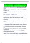
Lecture: The Keynesian Cross
model
Keynes’ theory: in the short run, P is
exogenous. Therefor focus on the
equilibrating forces in the goods market
(= how Y adjusts).
Model: closed economy in the short run,
to understand equilibrating forces in the goods market.
Closed economy: NX = 0
Equilibrium: Y = C + I + G
Focus on goods market => i exogenous
Short run => P exogenous So that π = 0
Planned aggregate expenditure E = C + I + G
Equilibrium if Y = E
Preparation: Chap 11: Aggregate Demand I: Building the
IS-LM Model
IS-LM model: Model of aggregate demand, leading interpretation of Keynes’
theory.
IS curve: Investment; “investment” and “saving” (market for goods and services)
LM curve: Saving; “liquidity” and “money” (supply and demand for money)
The IS curve plot is the relationship between the interest rate and the level of
income that arises in the market for goods and services.
The Keynesian cross: simplest interpretation of Keynes’s theory of how national
income is determined and is a building block for IS-LM Model.
Actual expenditure: amount households, firms and gov spend on goods and
services = GDP
Planned expenditure: amount the previous would like to spend on goods and
services.
PE = C + I + G
PE = C (Y – T) + I + G
Assumption: The economy is in equilibrium when actual expenditure = planned
expenditure.
So Y = PE
∆Y/∆G is the government-purchases multiplier.
When a government purchase raises income, it raises consumption as well.
∆Y/∆G = 1/(1 – MPC)
∆Y/∆T = - MPC / (1 – MPC) = Tax Multiplier
I = I(r)
The IS curve shows the combinations of the interest rate and the level of
income that are consistent with equilibrium in the market for goods and
services. The IS curve is drawn for a given fiscal policy. Changes in fiscal
policy that raise the demand for goods and services shift the IS curve to
the right. Changes in fiscal policy that reduce the demand for goods and
services shift the IS curve to the left.
Theory of liquidity preference: a theory of the interest rate.
(M/P)S = M/ P
(M/P)d= L(r)
(M/P)d= L(r, Y)
The LM curve shows the combinations of the interest rate and the level of
income that are consistent with equilibrium in the market for real money
balances. The LM curve is drawn for a given supply of real money
balances. Decreases in the supply of real money balances shift the LM
curve upward. Increases in the supply of real money balances shift the LM
curve downward.
, Chap 12: Aggregate Demand II: Applying the IS-
LM Model
Monetary transmission mechanism: how a monetary expansion induces greater
spending on goods and services.
IS-LM model shows that an increase in the money supply lowers the interest rate,
which stimulates investment and thereby expands the demand for goods and
services.
A macroeconometric model is a model that describes the economy
quantitatively, rather than just qualitatively.
Assumptions about monetary policy:
- The Fed keeps the nominal interest rate constant
- The Fed keeps the money supply constant so that the LM curve does not
shift.
According to Keynes, some changes like shocks to the IS curve can arise from
investors’ animal spirits or pessimism.
Shocks in the LM curve arise from exogenous changes in the demand for money.
Federal fund rate: The interest rate that banks charge one another for overnight
loans -> Short-term policy instrument.
A change in income in th IS-LM model resulting from a change in the price
level represents a movement along the aggregate demand curve. A
change in income in the IS-LM model for a given price level represents a
shift in the aggregate demand curve.
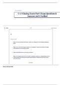
Lecture: The Keynesian Cross
model
Keynes’ theory: in the short run, P is
exogenous. Therefor focus on the
equilibrating forces in the goods market
(= how Y adjusts).
Model: closed economy in the short run,
to understand equilibrating forces in the goods market.
Closed economy: NX = 0
Equilibrium: Y = C + I + G
Focus on goods market => i exogenous
Short run => P exogenous So that π = 0
Planned aggregate expenditure E = C + I + G
Equilibrium if Y = E