Statistics and Mathematics
Lec. 1: Variables, Measurement levels,
Distributions
- Manifest variables
o give observable/ factual information
o only one question needed to get this information
o examples: age, gender, education level, holiday destination,…
- Latent variables:
o give non-observable information (opposite of Manifest variables)
o many questions needed to get this information
o examples: attitudes, satisfaction, beliefs and characteristics
- Content validity: Do different items cover all the contents of the construct to be measured?
- Construct validity: Does the measurement scale reflect theoretical position regarding a
construct?
- Measurement levels:
Nominal scale Categorical variable
Ordinal scale = can be devided into existing categories
Interval scale Continous variable =
Ration scale “real numbers“
- Measures of central tendency: Mean = average → hypothetical value (you
cannot have
└> middle point of distribution 2,6 friends)
Median = 0, 1, 1, 3, ④, 4, 4, 5, 5
Mode = most frequently mode 0, 1, 1, 3, 4, 4, 4, 5, 5
Lec. 2: Distributions and how to describe them
- Dispersion = how values differ from the mean → variation/ variance
between values
- Proportion (p): e.g. total 25
Males 6 𝑝=
Female 19
- Variance ration (VR): e.g. 𝑉𝑅 = 1 − ( ) VR = 1-p
VR=0 No variance VR=1 Variance in the
data
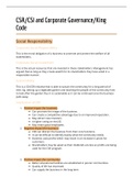
- Interquartile range:
n
SS
- Mean squared error (MS): Ms= =∑ ¿ ¿ ¿
df i=1
, √∑
n
- Standard deviation (SD or s(x) or sₓ): SD= ¿¿¿¿¿
i=1
- Represents:
o “fit“ of mean to data
o Error
o variability in the data
Nominal Mode Variance ratio Bar chart Pie
Ordinal Mode Mean Variance ratio chart
Interquartile range
Interval/Ratio → Mode Variance ratio Line diagram
scale in SPSS Mean Interquartile range Boxplot
Median Standard deviation Histogram
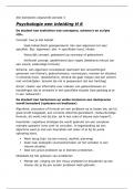
- Deviations from normality
o
o Pos. kurtosis = leptokurtic Neg.
kurtosis = platykurtic
, ➢ SPSS
• Compute general things of your data
→ Analyze
→ Descriptive statistics
→ Descriptives
→ Select the variable of which you want the analysis
→ Select under Options what you want to calculate
• Plot the data
→ Graphs
→ Chart builder
→ Select the way it should be plotted (Pie, Line, Bar,…) by moving your option into the big
field
→ Define the axis by moving the variables to the right axis
• Create new variable
→ Transform
→ Compute variable
→ Give your new variable a name under “Target variable”
→ add the variables of which you want to have a new one and divide them by the number
of variables
you used (e.g. (vari1 + vari2 + vari3 + vari4 + vari5) : 5 )
• Select variables
→ Data
→ Select cases
→ Select “if condition is satisfied”
→ Klick “If”
→ Select the variable that decides whether you keep it or not in your analysis
→ e.g. gender=1 means you keep all the data whose gender is 1…
o the others are not taken into account in your analysis
o (→ if you don’t what this selection anymore, click “data” → ”select cases”→
“All cases”)
, Lec. 3: The normal Distribution, the z-transform
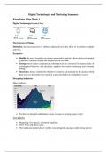
• Normal distribution:
o used to predict probabilities that given score occurs
1 (x−μ)2
o f ( x , μ ,σ )= e−
σ √2 π 2σ
2
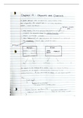
x i− x
Z-transform: Zi
Sx
afterwards: Mean = 0 SD = 1
SPSS:
o P-P Plot
o Analyze
o Descriptive statistics
o P-P plots
o Select the variable you want
o OK
• Skewness and kurtosis
→ Analyze
→ Descriptive statistics
→ Frequencies
→ Select under Statistics what you want to calculate (e.g. skewness & kurtosis)
• K-S test (Kolmogorov-Smirnov-test)
→ Analyze
→ Descriptive statistics
→ Explore
→ select the variable and put it in “dependent list”
→ Plots
→ Normality plots with tests
Lec. 4: Probability theory
e.g. 6 cups to evaluate whether tea was first given into the cup (TF) or the milk first (MF)7 └>
chance of haveing all right 0,5⁶= 0,015625
AND rule of probability:
o independent events
o e.g. role 2 on 1st dice AND role 2 on 2nd dice
▪ ⅙ ∙ ⅙
▪ Pr (A=a, B=b) = Pr(A=a) ∙ Pr(B=b)
OR rule of probability:
o e.g. role 2 a OR a 3 on a die
⅙ + ⅙
NOT rule of probability:
o e.g. not role a 2 on a die
Lec. 1: Variables, Measurement levels,
Distributions
- Manifest variables
o give observable/ factual information
o only one question needed to get this information
o examples: age, gender, education level, holiday destination,…
- Latent variables:
o give non-observable information (opposite of Manifest variables)
o many questions needed to get this information
o examples: attitudes, satisfaction, beliefs and characteristics
- Content validity: Do different items cover all the contents of the construct to be measured?
- Construct validity: Does the measurement scale reflect theoretical position regarding a
construct?
- Measurement levels:
Nominal scale Categorical variable
Ordinal scale = can be devided into existing categories
Interval scale Continous variable =
Ration scale “real numbers“
- Measures of central tendency: Mean = average → hypothetical value (you
cannot have
└> middle point of distribution 2,6 friends)
Median = 0, 1, 1, 3, ④, 4, 4, 5, 5
Mode = most frequently mode 0, 1, 1, 3, 4, 4, 4, 5, 5
Lec. 2: Distributions and how to describe them
- Dispersion = how values differ from the mean → variation/ variance
between values
- Proportion (p): e.g. total 25
Males 6 𝑝=
Female 19
- Variance ration (VR): e.g. 𝑉𝑅 = 1 − ( ) VR = 1-p
VR=0 No variance VR=1 Variance in the
data
- Interquartile range:
n
SS
- Mean squared error (MS): Ms= =∑ ¿ ¿ ¿
df i=1
, √∑
n
- Standard deviation (SD or s(x) or sₓ): SD= ¿¿¿¿¿
i=1
- Represents:
o “fit“ of mean to data
o Error
o variability in the data
Nominal Mode Variance ratio Bar chart Pie
Ordinal Mode Mean Variance ratio chart
Interquartile range
Interval/Ratio → Mode Variance ratio Line diagram
scale in SPSS Mean Interquartile range Boxplot
Median Standard deviation Histogram
- Deviations from normality
o
o Pos. kurtosis = leptokurtic Neg.
kurtosis = platykurtic
, ➢ SPSS
• Compute general things of your data
→ Analyze
→ Descriptive statistics
→ Descriptives
→ Select the variable of which you want the analysis
→ Select under Options what you want to calculate
• Plot the data
→ Graphs
→ Chart builder
→ Select the way it should be plotted (Pie, Line, Bar,…) by moving your option into the big
field
→ Define the axis by moving the variables to the right axis
• Create new variable
→ Transform
→ Compute variable
→ Give your new variable a name under “Target variable”
→ add the variables of which you want to have a new one and divide them by the number
of variables
you used (e.g. (vari1 + vari2 + vari3 + vari4 + vari5) : 5 )
• Select variables
→ Data
→ Select cases
→ Select “if condition is satisfied”
→ Klick “If”
→ Select the variable that decides whether you keep it or not in your analysis
→ e.g. gender=1 means you keep all the data whose gender is 1…
o the others are not taken into account in your analysis
o (→ if you don’t what this selection anymore, click “data” → ”select cases”→
“All cases”)
, Lec. 3: The normal Distribution, the z-transform
• Normal distribution:
o used to predict probabilities that given score occurs
1 (x−μ)2
o f ( x , μ ,σ )= e−
σ √2 π 2σ
2
x i− x
Z-transform: Zi
Sx
afterwards: Mean = 0 SD = 1
SPSS:
o P-P Plot
o Analyze
o Descriptive statistics
o P-P plots
o Select the variable you want
o OK
• Skewness and kurtosis
→ Analyze
→ Descriptive statistics
→ Frequencies
→ Select under Statistics what you want to calculate (e.g. skewness & kurtosis)
• K-S test (Kolmogorov-Smirnov-test)
→ Analyze
→ Descriptive statistics
→ Explore
→ select the variable and put it in “dependent list”
→ Plots
→ Normality plots with tests
Lec. 4: Probability theory
e.g. 6 cups to evaluate whether tea was first given into the cup (TF) or the milk first (MF)7 └>
chance of haveing all right 0,5⁶= 0,015625
AND rule of probability:
o independent events
o e.g. role 2 on 1st dice AND role 2 on 2nd dice
▪ ⅙ ∙ ⅙
▪ Pr (A=a, B=b) = Pr(A=a) ∙ Pr(B=b)
OR rule of probability:
o e.g. role 2 a OR a 3 on a die
⅙ + ⅙
NOT rule of probability:
o e.g. not role a 2 on a die