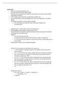
Sticky prices
- Short-term upward-sloping AS curve
- The basis of new Keynesian DSGE models
- These are the most widely used models of the business cycle used in central banks
and academic research
- These models assume that firms cannot always change price
- In our version there Is a fixed probability that a firm can change price in any given
period
- Our analysis is based on a classic paper by Mankiw
o The inexorable and mysterious trade-off between inflation and
unemployment
- Suppose there is a 50/50 chance a firm can change price
- The probability of being able to change prices is λ=0.5
- Assume that firms are identical, apart from the fact that in any period, 50% of firms
can change price and 50% cannot
- Notation
o p is the log of the price level
o x is the log of the price chosen by firms that are able to change price
o p* is the log of the price that firms would choose if they could change price in
every period
- underlying the model Is some complicated algebra
- all firms that can change price will choose the same price
o λ = 50% of firms can change their price in this period. They all choose the
same price: Xt
o λ(1- λ) = 25% of firms were able to change their price in the previous period
but cannot change it in this period. In the previous period these firms all
choose the. Same price: Xt-1
o λ(1- λ)^2 = 12.5% of firms were able to change their price two periods ago
but were not able to change their price since then. two periods ago these
firms changed the same price: Xt-2
o λ(1- λ)^3 = 6.25% of firms were able to change their price three periods ago
but were not able to change their price since then three periods ago these
firms changed the same price: Xt-3
o ect
- the (log) price level is
o pt= 0.5Xt + 0.25Xt-1 + 0.125Xt-2 + 0.0625Xt-3 + …..
assuming λ = 0.5
o in general
, 2 3
pt = λxt + λ(1 − λ)xt−1 + λ(1 − λ) xt−2 + λ(1 − λ) xt−3 + ...
o in mathematical notation
1
- Assuming λ = 0.5, what price will firms choose
- Suppose a firms preferred price in period t is pt*
o λ = 50% of firms can change their price in this period. Their preferred price in
this period is pt*
o λ(1-λ) = 25% of firms can change their price in this period but will not be able
to change their price in period t + 1. Their preferred price in period t + 1 will
be pt+1*. Firms don’t know this in period t, so they use the expected value:
Etpt+1*
o λ(1-λ)^2 = 12.5% of firms can change their price in this period but will not be
able to change their price in either period t + 1 or period t + 2. Their preferred
price in period t + 2 will be pt+2*. Firms don’t know this in period t, so they
use the expected value: Etpt+2*
o etc
- the price chosen by firms is therefore
o
o This assumes λ = 0.5
- In general

