Applied Financial Econometrics
Summary of the Lectures
University of Amsterdam
MSc Finance
2022
,Week 1 - OLS and Experiments
Part B: OLS & Endogeneity
What you should already know: Ordinary Least Squares or “doing a regression”
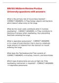
OLS: Drawing a line through data (Ch4; p146[159])
It is called OLS because Stata draws a line through the points such that the sum of the squares
residuals (difference from predicted line) is minimal.
OLS estimator formulas
● B1 hat is the slope of the line. Sxy is the sample covariance of the dataset. S2x is the sample
variance of x. You should know this formula!
● Second formula is the intercept of the line. You should know this formula!
1
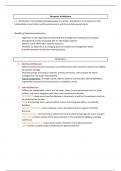
,OLS: testing and interpreting a slope coefficient (Ch7 & 8)
● If schooling goes up with one year, income increases 16.52%.
● T-statistic = coëfficiënt / standard error = 0..0083 = 19.86.
○ 19.86 > 1.96 meaning that there is a relationship.
● P value = 0.000 -> chance that coefficient in another sample is 0.1653 and there is no relation
between schooling and wage.
OLS: Core assumptions
The following 3 core assumptions must hold:
1. X does not move with u. The mean of u will be 0.
2. Sample must be random e.g. not only sampling from high education people.
3. The tales of the variables should go to 0 quickly enough e.g. you can't have negative earnings
(natually bounded) so that is okay.
2
,OLS: Consistency
Consistency: what if we take the entire population, will it still hold?
Covariance rules:
● Because B1 is a constant, you can put it in front.
● Because B0 is a constant, the covariance between X and B0 is 0.
So when you calculate your B1hat you get the B1 + formula and you hope that is as small as possible
and it will be 0 as assumption 1 holds!
What you (hopefully) already know: Ordinary Least Squares Inconsistency
When is OLS consistent?
Endogeneity leads to OLS inconsistency
● Even when you take the whole population as sample, you get B1 + *formula* because X is
correlated with u.
● Positive selection: *formula is positive - > overestimation of B1
● Negative selection: *formula is negative -> underestimation of B1
3
,Observational (just random sample) Data in general
Sources of endogeneity: 4 situations
● Omitted variables: if y1cov(xi,Wi) is not 0, then cov (X,u) is also not 0, meaning that we have
endogeneity by some omitted variable W. Only the W that are related to Y cause problems!
● Reversed causality: X causes Y and Y causes X.
○ To get the the cov formula on the bottom right: plug Xi in with ui. y0 and B0 are
constants. ni has 0 covariance with ui (bottom left).
○ We get reversed causality problems when: the y1 is not 0!
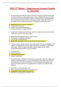
Example: Reversed causality in the knowledge-about and the use-of student loans
Knowledge about student loans and loan take-up
When a students loans more -> students learn more
OR
When a student leans more -> students loan more
4
,Does knowledge increase loan take-up?
Or does loan take-up increase knowledge?
Part C: Potential Outcomes
Causal Effects
● Treatment variable because you “treat” the sample with X.
5
,Potential outcomes
● Example: getting a MSc degree or not for each individual i and then taking the average ->
ATE
Potential outcomes example: loan take-up and knowledge
Person 1 is not borrowing even when given more information -> Treatment effect is 0.
If everybody is given more information 25% will borrow. Same for not giving more information.
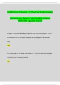
The counterfactual problem
What would have happened if Robben scored? -> other state of the world.
6
,● The question marks are the counterfactuals.
● If we used this dataset, we would believe that the ATE would be 0.50.
7
,The counterfactual problem: Solve by OLS?
● Homogeneous treatment effect: effect is the same for everyone
● If X is 0 you observe Y0, if X is 1 you observe Y1.
● You add E(Y(0)) to get a B0. This is the average Y if nobody received the treatment And then
you also subtract it because otherwise you modify the equation.
● B1 measures the improvement if everyone gets the treatment.
● ui measures if the individual is below or above average.
● In this case there is an upward bias as the *formula* next to B1 is positive (0.5) -> exogeneity
does not hold.
The counterfactual problem and endogeneity: in a graph
Identification: Solutions to the counterfactual problem
● Experimental: you manipulate X variable and randomly assign people
● Observational: not changing just observing (from gotten sample) assuming random sample
8
, Part D: Experiments - Design
Identification using experimental data
● Randomized Control Trail (RCT): randomly assign individuals with X=1 or X=0. In this way
you eliminate all endogeneity.
● Spillovers: what happens to someone, happens also to somebody else because of that.
2 ways of achieving exogeneity by construction
Unconditional Random assignment
● Randomly decide if a person receives treatment.
Conditional Random assignment
9
Summary of the Lectures
University of Amsterdam
MSc Finance
2022
,Week 1 - OLS and Experiments
Part B: OLS & Endogeneity
What you should already know: Ordinary Least Squares or “doing a regression”
OLS: Drawing a line through data (Ch4; p146[159])
It is called OLS because Stata draws a line through the points such that the sum of the squares
residuals (difference from predicted line) is minimal.
OLS estimator formulas
● B1 hat is the slope of the line. Sxy is the sample covariance of the dataset. S2x is the sample
variance of x. You should know this formula!
● Second formula is the intercept of the line. You should know this formula!
1
,OLS: testing and interpreting a slope coefficient (Ch7 & 8)
● If schooling goes up with one year, income increases 16.52%.
● T-statistic = coëfficiënt / standard error = 0..0083 = 19.86.
○ 19.86 > 1.96 meaning that there is a relationship.
● P value = 0.000 -> chance that coefficient in another sample is 0.1653 and there is no relation
between schooling and wage.
OLS: Core assumptions
The following 3 core assumptions must hold:
1. X does not move with u. The mean of u will be 0.
2. Sample must be random e.g. not only sampling from high education people.
3. The tales of the variables should go to 0 quickly enough e.g. you can't have negative earnings
(natually bounded) so that is okay.
2
,OLS: Consistency
Consistency: what if we take the entire population, will it still hold?
Covariance rules:
● Because B1 is a constant, you can put it in front.
● Because B0 is a constant, the covariance between X and B0 is 0.
So when you calculate your B1hat you get the B1 + formula and you hope that is as small as possible
and it will be 0 as assumption 1 holds!
What you (hopefully) already know: Ordinary Least Squares Inconsistency
When is OLS consistent?
Endogeneity leads to OLS inconsistency
● Even when you take the whole population as sample, you get B1 + *formula* because X is
correlated with u.
● Positive selection: *formula is positive - > overestimation of B1
● Negative selection: *formula is negative -> underestimation of B1
3
,Observational (just random sample) Data in general
Sources of endogeneity: 4 situations
● Omitted variables: if y1cov(xi,Wi) is not 0, then cov (X,u) is also not 0, meaning that we have
endogeneity by some omitted variable W. Only the W that are related to Y cause problems!
● Reversed causality: X causes Y and Y causes X.
○ To get the the cov formula on the bottom right: plug Xi in with ui. y0 and B0 are
constants. ni has 0 covariance with ui (bottom left).
○ We get reversed causality problems when: the y1 is not 0!
Example: Reversed causality in the knowledge-about and the use-of student loans
Knowledge about student loans and loan take-up
When a students loans more -> students learn more
OR
When a student leans more -> students loan more
4
,Does knowledge increase loan take-up?
Or does loan take-up increase knowledge?
Part C: Potential Outcomes
Causal Effects
● Treatment variable because you “treat” the sample with X.
5
,Potential outcomes
● Example: getting a MSc degree or not for each individual i and then taking the average ->
ATE
Potential outcomes example: loan take-up and knowledge
Person 1 is not borrowing even when given more information -> Treatment effect is 0.
If everybody is given more information 25% will borrow. Same for not giving more information.
The counterfactual problem
What would have happened if Robben scored? -> other state of the world.
6
,● The question marks are the counterfactuals.
● If we used this dataset, we would believe that the ATE would be 0.50.
7
,The counterfactual problem: Solve by OLS?
● Homogeneous treatment effect: effect is the same for everyone
● If X is 0 you observe Y0, if X is 1 you observe Y1.
● You add E(Y(0)) to get a B0. This is the average Y if nobody received the treatment And then
you also subtract it because otherwise you modify the equation.
● B1 measures the improvement if everyone gets the treatment.
● ui measures if the individual is below or above average.
● In this case there is an upward bias as the *formula* next to B1 is positive (0.5) -> exogeneity
does not hold.
The counterfactual problem and endogeneity: in a graph
Identification: Solutions to the counterfactual problem
● Experimental: you manipulate X variable and randomly assign people
● Observational: not changing just observing (from gotten sample) assuming random sample
8
, Part D: Experiments - Design
Identification using experimental data
● Randomized Control Trail (RCT): randomly assign individuals with X=1 or X=0. In this way
you eliminate all endogeneity.
● Spillovers: what happens to someone, happens also to somebody else because of that.
2 ways of achieving exogeneity by construction
Unconditional Random assignment
● Randomly decide if a person receives treatment.
Conditional Random assignment
9