5. EXERCISE SESSION 1
5.1 INTEREST RATES
Exercise 1
An investor receives €1 100 in 1 year in return for an investment of €1000 now. Compounding:
Calculate the percentage return per annum with:
( )
m× t
Rm
1. Annual compounding: m = 1 1+
1100 m
1100=1000. ( 1+ R )=¿ R= −1=0.1=10 %
1000
2. Semiannual compounding: m = 2
1100=1000. 1+ ( ) R 2
2
=¿ R=2 × (√ 1100
1000
−1 )=9.7618 %
3. Monthly compounding: m = 12
( ) =¿ R=12× ( √ 1100 −1 )=9.5690 %
12
R 12
1100=1000. 1+
12 1000
4. Daily compounding: m = 365
( ) ( √ 1100 −1 )=9.5323 %
365
R 365
1100=1000. 1+ =¿ R=365 ×
365 1000
5. Continuous compounding: m = ∞
1100=1000× e =¿ R=ln
R
( 1100
1000 )
=9.5310 %
Exercise 2
Given zero coupon interest rates in quarterly compounding:
1. Compute the discount factors using the quarterly compounding rates:
1%
=0.25 % = quarterly rate
4
1 = Term structure
With annual compounding m=1: Discount factor=
1+1 %
1
Discount factor for 1 years= =0.990062
1+
1% 4
4 ( )
1
Discount factor for 2 years= =0.9608
( )
8
2%
1+
4
1
Discount factor for 3 years= =0.914238
( )
12
3%
1+
4
1
Discount factor for 4 years= =0.852821
( )
16
4%
1+
4
2. Convert the rates to continuous compounding:
( ) [( ) ] [ ]
m× t m
Rm RC × t Rm Rm
1+ =e =¿ RC =ln 1+ = ¿ R C =m ×ln 1+
m m m
1 years: R C =4 × ln 1+
0.01
4 [
=0.99875 %
]
2 years: RC =4 × ln 1+
0.02
4 [
=1.99502%
]
, 3 years: RC =4 × ln 1+
0.03
4 [=2.988806 %
]
4 years: RC =4 × ln 1+
0.04
4 [=3.98013 %
]
3. Compute the discount factors starting from the rates in continuous compounding:
We’ll get the exact same answers as question 1, because we computed the equivalent rates.
4. Compute the forward rate for the period year 2 and 3 in continuous compounding:
R 2C × 2 f 2,3 ×1 R3 C ×3
e ×e =e
¿> f 2,3 =R 3 C × 3−R2 C ×2=2.988806 % ×3−1.99502% ×2=4.976378 %
Exercise 3
Suppose that the forward SOFR rate for the period between time 1.5 years and time 2 years in the future is
5% (with semiannual compounding) and that some time ago a company entered into an FRA where it will
receive 5.8% (with semiannual compounding) and pay SOFR on a principal of $100 million for the period.
The 2-year SOFR risk-free rate is 4% (with continuous compounding). What is the value of the FRA?
FRA → FR A 0=PV [ τ ( R K −R F ) L ] of PV [τ ( RF −R K ) L]
τ =time , L=principal , ( R F−R K )∨( R K −R F )=difference between the ¿∧floating rate
( 100 000 000 [ 0.058−0.05 ] 0.5 ) × e−0.04 ×2=369 200
5.2 RISK MEASUREMENT
Exercise 1
Consider a position consisting of a €300 000 investment in gold and a €500 000 investment in silver.
Suppose that the daily volatilities of these 2 assets are 1.8% and 1.2% respectively, and that the coefficient
of correlation between their returns is 0.6.
We make the assumptions: normal distribution and zero means.
1. What is the 10-day 99% VaR for the portfolio?
−1
VaR=σ . N ( X ) . ¿ ¿
Va R portfolio =σ portfolio . N−1 ( X ) .¿ ¿
We still need to compute the standard deviation of the total portfolio.
Cov ( X ,Y )
Var ( aX +bY ) =a2 Var ( X )+ b2 Var ( Y ) +2 abCov (X , Y ) & ρ=
σ X σY
¿> ()
3 2
8
2
.1.8 % +
5 2
8 () 2 3 5
.1.2 % + 2. . . 0.6 . 1.8 % . 1.2%
8 8
√( ) ()
2 2
3 5 3 5
σ p=√ Va r portfolio =
2 2
. 0.018 + . 0.012 + 2. . . 0.6 . 0.018 .0.012=0.01275
8 8 8 8
1−day VaR=0.01275 . N −1 ( 99 % ) .800000=0.01275 . 2.326 .800 000=€ 23725.20
10−day VaR=1−day VaR × √ 10=€ 75 025.67
2. By how much does diversification reduce the VaR?
ρ gs =1
Joint VaR=Va R1+ Va R 2=0.018 .2.326 . 300 000+0.012 . 2.326 .500 000
10−day VaR=( 0.018 . 2.326 .300 000+ 0.012. 2.326 .500 000 ) . √ 10=83 852.217
The benefits of diversification are €83 852.217 - €75 025.67.
5.1 INTEREST RATES
Exercise 1
An investor receives €1 100 in 1 year in return for an investment of €1000 now. Compounding:
Calculate the percentage return per annum with:
( )
m× t
Rm
1. Annual compounding: m = 1 1+
1100 m
1100=1000. ( 1+ R )=¿ R= −1=0.1=10 %
1000
2. Semiannual compounding: m = 2
1100=1000. 1+ ( ) R 2
2
=¿ R=2 × (√ 1100
1000
−1 )=9.7618 %
3. Monthly compounding: m = 12
( ) =¿ R=12× ( √ 1100 −1 )=9.5690 %
12
R 12
1100=1000. 1+
12 1000
4. Daily compounding: m = 365
( ) ( √ 1100 −1 )=9.5323 %
365
R 365
1100=1000. 1+ =¿ R=365 ×
365 1000
5. Continuous compounding: m = ∞
1100=1000× e =¿ R=ln
R
( 1100
1000 )
=9.5310 %
Exercise 2
Given zero coupon interest rates in quarterly compounding:
1. Compute the discount factors using the quarterly compounding rates:
1%
=0.25 % = quarterly rate
4
1 = Term structure
With annual compounding m=1: Discount factor=
1+1 %
1
Discount factor for 1 years= =0.990062
1+
1% 4
4 ( )
1
Discount factor for 2 years= =0.9608
( )
8
2%
1+
4
1
Discount factor for 3 years= =0.914238
( )
12
3%
1+
4
1
Discount factor for 4 years= =0.852821
( )
16
4%
1+
4
2. Convert the rates to continuous compounding:
( ) [( ) ] [ ]
m× t m
Rm RC × t Rm Rm
1+ =e =¿ RC =ln 1+ = ¿ R C =m ×ln 1+
m m m
1 years: R C =4 × ln 1+
0.01
4 [
=0.99875 %
]
2 years: RC =4 × ln 1+
0.02
4 [
=1.99502%
]
, 3 years: RC =4 × ln 1+
0.03
4 [=2.988806 %
]
4 years: RC =4 × ln 1+
0.04
4 [=3.98013 %
]
3. Compute the discount factors starting from the rates in continuous compounding:
We’ll get the exact same answers as question 1, because we computed the equivalent rates.
4. Compute the forward rate for the period year 2 and 3 in continuous compounding:
R 2C × 2 f 2,3 ×1 R3 C ×3
e ×e =e
¿> f 2,3 =R 3 C × 3−R2 C ×2=2.988806 % ×3−1.99502% ×2=4.976378 %
Exercise 3
Suppose that the forward SOFR rate for the period between time 1.5 years and time 2 years in the future is
5% (with semiannual compounding) and that some time ago a company entered into an FRA where it will
receive 5.8% (with semiannual compounding) and pay SOFR on a principal of $100 million for the period.
The 2-year SOFR risk-free rate is 4% (with continuous compounding). What is the value of the FRA?
FRA → FR A 0=PV [ τ ( R K −R F ) L ] of PV [τ ( RF −R K ) L]
τ =time , L=principal , ( R F−R K )∨( R K −R F )=difference between the ¿∧floating rate
( 100 000 000 [ 0.058−0.05 ] 0.5 ) × e−0.04 ×2=369 200
5.2 RISK MEASUREMENT
Exercise 1
Consider a position consisting of a €300 000 investment in gold and a €500 000 investment in silver.
Suppose that the daily volatilities of these 2 assets are 1.8% and 1.2% respectively, and that the coefficient
of correlation between their returns is 0.6.
We make the assumptions: normal distribution and zero means.
1. What is the 10-day 99% VaR for the portfolio?
−1
VaR=σ . N ( X ) . ¿ ¿
Va R portfolio =σ portfolio . N−1 ( X ) .¿ ¿
We still need to compute the standard deviation of the total portfolio.
Cov ( X ,Y )
Var ( aX +bY ) =a2 Var ( X )+ b2 Var ( Y ) +2 abCov (X , Y ) & ρ=
σ X σY
¿> ()
3 2
8
2
.1.8 % +
5 2
8 () 2 3 5
.1.2 % + 2. . . 0.6 . 1.8 % . 1.2%
8 8
√( ) ()
2 2
3 5 3 5
σ p=√ Va r portfolio =
2 2
. 0.018 + . 0.012 + 2. . . 0.6 . 0.018 .0.012=0.01275
8 8 8 8
1−day VaR=0.01275 . N −1 ( 99 % ) .800000=0.01275 . 2.326 .800 000=€ 23725.20
10−day VaR=1−day VaR × √ 10=€ 75 025.67
2. By how much does diversification reduce the VaR?
ρ gs =1
Joint VaR=Va R1+ Va R 2=0.018 .2.326 . 300 000+0.012 . 2.326 .500 000
10−day VaR=( 0.018 . 2.326 .300 000+ 0.012. 2.326 .500 000 ) . √ 10=83 852.217
The benefits of diversification are €83 852.217 - €75 025.67.