,
,Q2: Follow up the data on Q1. Use the R pipeline to build the linear regression model. Compare the
result from R and the result by your manual calculation.
Solution:
data = rbind(c(-0.15, -0.48, 0.46),c(-0.72, -0.54, -0.37),c(1.36, -0.91, -0.2
7),c(0.61, 1.59, 1.35),c(-1.11, 0.34, -0.11))
data = data.frame(data)
names(data)
## [1] "X1" "X2" "X3"
colnames(data) = c("X1","X2","Y")
lm.YX <-lm(Y~X1+X2,data = data)
summary(lm.YX)
2
, ##
## Call:
## lm(formula = Y ~ X1 + X2, data = data)
##
## Residuals:
## 1 2 3 4 5
## 0.5663 -0.1014 -0.2435 0.0566 -0.2780
##
## Coefficients:
## Estimate Std. Error t value Pr(>|t|)
## (Intercept) 0.2124 0.2170 0.979 0.431
## X1 0.2222 0.2430 0.914 0.457
## X2 0.5946 0.2430 2.447 0.134
##
## Residual standard error: 0.4852 on 2 degrees of freedom
## Multiple R-squared: 0.7682, Adjusted R-squared: 0.5365
## F-statistic: 3.315 on 2 and 2 DF, p-value: 0.2318
Q3: Please read the following output in R.
(1) Write up the fitted regression model.
(2) Identify the significant variables.
(3) What is the R-squared of this model? Does the model fit the data well?
(4) What would you recommend as the next step in data analysis?
##
## Call:
## lm(formula = y ~ ., data = data)
##
## Residuals:
## Min 1Q Median 3Q Max
## -0.239169 -0.065621 0.005689 0.064270 0.310456
##
## Coefficients:
## Estimate Std. Error t value Pr(>|t|)
## (Intercept) 0.009124 0.010473 0.871 0.386
## x1 1.008084 0.008696 115.926 <2e-16 ***
## x2 0.494473 0.009130 54.159 <2e-16 ***
## x3 0.012988 0.010055 1.292 0.200
## x4 -0.002329 0.009422 -0.247 0.805
## ---
## Signif. codes: 0 '***' 0.001 '**' 0.01 '*' 0.05 '.' 0.1 ' ' 1
##
## Residual standard error: 0.1011 on 95 degrees of freedom
## Multiple R-squared: 0.9942, Adjusted R-squared: 0.994
## F-statistic: 4079 on 4 and 95 DF, p-value: < 2.2e-16
3
,Q2: Follow up the data on Q1. Use the R pipeline to build the linear regression model. Compare the
result from R and the result by your manual calculation.
Solution:
data = rbind(c(-0.15, -0.48, 0.46),c(-0.72, -0.54, -0.37),c(1.36, -0.91, -0.2
7),c(0.61, 1.59, 1.35),c(-1.11, 0.34, -0.11))
data = data.frame(data)
names(data)
## [1] "X1" "X2" "X3"
colnames(data) = c("X1","X2","Y")
lm.YX <-lm(Y~X1+X2,data = data)
summary(lm.YX)
2
, ##
## Call:
## lm(formula = Y ~ X1 + X2, data = data)
##
## Residuals:
## 1 2 3 4 5
## 0.5663 -0.1014 -0.2435 0.0566 -0.2780
##
## Coefficients:
## Estimate Std. Error t value Pr(>|t|)
## (Intercept) 0.2124 0.2170 0.979 0.431
## X1 0.2222 0.2430 0.914 0.457
## X2 0.5946 0.2430 2.447 0.134
##
## Residual standard error: 0.4852 on 2 degrees of freedom
## Multiple R-squared: 0.7682, Adjusted R-squared: 0.5365
## F-statistic: 3.315 on 2 and 2 DF, p-value: 0.2318
Q3: Please read the following output in R.
(1) Write up the fitted regression model.
(2) Identify the significant variables.
(3) What is the R-squared of this model? Does the model fit the data well?
(4) What would you recommend as the next step in data analysis?
##
## Call:
## lm(formula = y ~ ., data = data)
##
## Residuals:
## Min 1Q Median 3Q Max
## -0.239169 -0.065621 0.005689 0.064270 0.310456
##
## Coefficients:
## Estimate Std. Error t value Pr(>|t|)
## (Intercept) 0.009124 0.010473 0.871 0.386
## x1 1.008084 0.008696 115.926 <2e-16 ***
## x2 0.494473 0.009130 54.159 <2e-16 ***
## x3 0.012988 0.010055 1.292 0.200
## x4 -0.002329 0.009422 -0.247 0.805
## ---
## Signif. codes: 0 '***' 0.001 '**' 0.01 '*' 0.05 '.' 0.1 ' ' 1
##
## Residual standard error: 0.1011 on 95 degrees of freedom
## Multiple R-squared: 0.9942, Adjusted R-squared: 0.994
## F-statistic: 4079 on 4 and 95 DF, p-value: < 2.2e-16
3