Laura van den End
0. Introduction
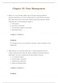
Cases and variables Variance and standard deviation
Cases: sampling unit - individuals Variance: σ2 (pop variance) or s2 (sample variance)
- Average squared deviation form the mean
Response variable: dependent outcome
- Measured variable you want to explain in function Length Dev from mean Squared dev
of the predictor variables - species abundances, from mean
gene expression, mortality
5 2 4
Predictor variable: independent variable
- Measured variable to help explain variation in 2 -1 1
response variable - pH, nutrient abundance, 2 -1 1
environmental conditions, body size, age
2 0 3
Types of variables
Categorical: non-numerical, factors 3 0 2
- Exp. treatment, sex → have discrete levels
Standard deviation: σ (pop) or s (sample) = √variance
Continuous: scale
- Body size, weight, pH, concentration, time
Percentiles
Value of variable below which x% of values lie
Count: integer - e.g 25% of the data lay below the 25th percentile
- Number of offspring, species abundance - Interquartile range: range between 25th and 75th
percentile
Ordinal:
- Preference on a scale from 1-7
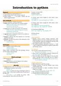
The normal distribution
- Common distribution for continuous data
Descriptive vs inferential statistics - Bell-shaped, symmetrical around µ= x
Descriptive statistics: describe the data - Mean µ ± 1.96 * σ includes 95% of the observations
- Mean, standard deviation, correlation coefficient - Probability density function:
- Distribution of data, histograms, box plots
Inferential statistics: make inferences about a Skewness and kurtosis
population based on a sample Skewness: measure of asymmetry of distribution - 3rd
- Testing hypotheses with statistical tests standardized moment (mean = 1st moment, standard
- Calculating confidence intervals deviation = 2nd).
- Drawing conclusions
Kurtosis: pointless of the distribution - 4 th
standardized moment.
Descriptive statistics
(arithmetic) mean
- All values summed divided by # of observations The standard normal distribution
- Not informative for multimodal or asym distribut. A normal distribution with mean 0 and standard
- Sensitive to outliers deviation 1
Median ‘Standardizing’ your data means:
- Middle value if all values are ordered - Subtracting the mean
- Better summary statistic for asym distributed data - Dividing by the st.deviation
- Not sensitive to outliers - The resulting numbers are the
‘z-scores’ of your data points
Mode
- Value that appears most frequently in a data set
Advanced biological data analysis
, Laura van den End
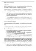
Inferential statistics
We want to draw general conclusions about a
population based on sample
- Sample: part of pop that you studied
- Pop: all cases you could have studied
Standard error
When we calculate a statistic of a sample (e.g. the
mean), this is an estimate of that statistic for the
population. If we would sample again, we would get
a slightly different estimate every time. The standard
error is the standard deviation of that statistic across
our different samples
This is a measure of the precision that we have in
estimating the actual population statistic. We can
actually calculate this standard error based on just a
single sample: with n = Sample size.
Standard deviation vs standard error
The standard deviation is a measure of spread in our
sample ~ higher = more variability in the data.
The standard error is a measure of precision ~ higher
= the lower confidence in the accuracy of estimate.
- More data (the higher n) = lower the SE
- Confidence intervals are based on the SE
Using statistics to test hypotheses
H0: no effect, Q: can we reject H0 → when small
change to get our data, assuming H0 is true
Types of errors
Type I error (false positive) - we reject a true H0
- This is expected to happen in 5% of the cases!
- Multiple testing increases frequency
Type II error (false negative) - don’t reject false H0
- e.g. because sample size is too low (not enough
statistical power)
Note: we never accept or confirm H0 – we only do or
do not reject it
Advanced biological data analysis
, Laura van den End
1. Linear models
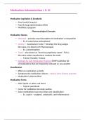
Continuous predictors Testing assumptions
STEP 1: visual inspection of raw data
> plot(body.length~heavy.metal.conc, data=caterpillars) Homogeneity of variances
STEP 2: regression line VISUALLY
- Draw the line → minimize the sum of squares of >spreadLevelPlot(fit3)
the difference between a datapoint and its - high absolute residuals = far away from reg. line
prediction - Low absolute residuals = close to regression line
- OLS - ordinaire least squares regression - We want equally distance. If the blue line is more
- Resulting line is given by 2 numbers: intercept and or less straight we have no problem.
slope:
TEST
>ncvTest(fit2)
STEP 3: fit a model → gives slope and intercept - If the p value is above 0.05 OK (no significant
> fit2 <- lm(body.length~heavy.metal.conc, data = data) deviation from homogeneous variances.
> summary(fit2)
NOT OK?
STEP 4: visualize results with effect plot - Transform data
>plot(allEffects(fit4), multiline = T, confint = list (style = - See if outliers
"auto")) - Use a model that allows for non-homogeneous
variances (gls)
STEP 5: hypothesis testing
- Take the summary table
- Take our confidence level given by SE Normality of residuals
- T value (estimate divided by SE) → more extreme
= less likely to get data if H0 is true VISUALLY
hist(rstudent(fit4), probability=T, ylim=c(0,0.5),
main="Distribution of Studentized Residuals",
Categorical predictors xlab="Studentized residuals”)
- Histogram of the studentized residuals of the
2 levels model
STEP 1 + 2 + 3 + 5: same
xfit=seq(-3,3, length=100)
STEP 4: same - Create a vector of X values for the normal
- R standard: ‘treatment coding’ = 1st alphabetical as distribution from -3 to 3
the reference level
- Sum coding → mean of all levels as reference level yfit=dnorm(xfit)
- Useful if collinearity in the data lines(xfit, yfit, col=“red”,lwd=2)
- Calculate and put values for a standard normal
More than 2 levels distribution of the range of x values given above
STEP 1 + 2 + 3 + 4: same
TEST
>shapiro.test(residuals(fit4))
STEP 5: check anova table for overall effect on the
- If W > 0.9 is OK
categorical predictor with more than 2 levels
> Anova(fit4, type=“III”)
Linearity
STEP 6: post-hoc comparisons >residualPlots(fit2)
- which levels of our predictor are different from - No strong relation is OK
each other?
> emmeans(fit4, ~samp.loc) Outliers and in uential observations
> contrast(emmeans(fit4, ~samp.loc), method='pairwise', > outlierTest(fit2) > cd <- cooks.distance(fit2)
adjust=‘Tukey’) > inflobs=which(cd>1);inflobs
Advanced biological data analysis
fl
0. Introduction
Cases and variables Variance and standard deviation
Cases: sampling unit - individuals Variance: σ2 (pop variance) or s2 (sample variance)
- Average squared deviation form the mean
Response variable: dependent outcome
- Measured variable you want to explain in function Length Dev from mean Squared dev
of the predictor variables - species abundances, from mean
gene expression, mortality
5 2 4
Predictor variable: independent variable
- Measured variable to help explain variation in 2 -1 1
response variable - pH, nutrient abundance, 2 -1 1
environmental conditions, body size, age
2 0 3
Types of variables
Categorical: non-numerical, factors 3 0 2
- Exp. treatment, sex → have discrete levels
Standard deviation: σ (pop) or s (sample) = √variance
Continuous: scale
- Body size, weight, pH, concentration, time
Percentiles
Value of variable below which x% of values lie
Count: integer - e.g 25% of the data lay below the 25th percentile
- Number of offspring, species abundance - Interquartile range: range between 25th and 75th
percentile
Ordinal:
- Preference on a scale from 1-7
The normal distribution
- Common distribution for continuous data
Descriptive vs inferential statistics - Bell-shaped, symmetrical around µ= x
Descriptive statistics: describe the data - Mean µ ± 1.96 * σ includes 95% of the observations
- Mean, standard deviation, correlation coefficient - Probability density function:
- Distribution of data, histograms, box plots
Inferential statistics: make inferences about a Skewness and kurtosis
population based on a sample Skewness: measure of asymmetry of distribution - 3rd
- Testing hypotheses with statistical tests standardized moment (mean = 1st moment, standard
- Calculating confidence intervals deviation = 2nd).
- Drawing conclusions
Kurtosis: pointless of the distribution - 4 th
standardized moment.
Descriptive statistics
(arithmetic) mean
- All values summed divided by # of observations The standard normal distribution
- Not informative for multimodal or asym distribut. A normal distribution with mean 0 and standard
- Sensitive to outliers deviation 1
Median ‘Standardizing’ your data means:
- Middle value if all values are ordered - Subtracting the mean
- Better summary statistic for asym distributed data - Dividing by the st.deviation
- Not sensitive to outliers - The resulting numbers are the
‘z-scores’ of your data points
Mode
- Value that appears most frequently in a data set
Advanced biological data analysis
, Laura van den End
Inferential statistics
We want to draw general conclusions about a
population based on sample
- Sample: part of pop that you studied
- Pop: all cases you could have studied
Standard error
When we calculate a statistic of a sample (e.g. the
mean), this is an estimate of that statistic for the
population. If we would sample again, we would get
a slightly different estimate every time. The standard
error is the standard deviation of that statistic across
our different samples
This is a measure of the precision that we have in
estimating the actual population statistic. We can
actually calculate this standard error based on just a
single sample: with n = Sample size.
Standard deviation vs standard error
The standard deviation is a measure of spread in our
sample ~ higher = more variability in the data.
The standard error is a measure of precision ~ higher
= the lower confidence in the accuracy of estimate.
- More data (the higher n) = lower the SE
- Confidence intervals are based on the SE
Using statistics to test hypotheses
H0: no effect, Q: can we reject H0 → when small
change to get our data, assuming H0 is true
Types of errors
Type I error (false positive) - we reject a true H0
- This is expected to happen in 5% of the cases!
- Multiple testing increases frequency
Type II error (false negative) - don’t reject false H0
- e.g. because sample size is too low (not enough
statistical power)
Note: we never accept or confirm H0 – we only do or
do not reject it
Advanced biological data analysis
, Laura van den End
1. Linear models
Continuous predictors Testing assumptions
STEP 1: visual inspection of raw data
> plot(body.length~heavy.metal.conc, data=caterpillars) Homogeneity of variances
STEP 2: regression line VISUALLY
- Draw the line → minimize the sum of squares of >spreadLevelPlot(fit3)
the difference between a datapoint and its - high absolute residuals = far away from reg. line
prediction - Low absolute residuals = close to regression line
- OLS - ordinaire least squares regression - We want equally distance. If the blue line is more
- Resulting line is given by 2 numbers: intercept and or less straight we have no problem.
slope:
TEST
>ncvTest(fit2)
STEP 3: fit a model → gives slope and intercept - If the p value is above 0.05 OK (no significant
> fit2 <- lm(body.length~heavy.metal.conc, data = data) deviation from homogeneous variances.
> summary(fit2)
NOT OK?
STEP 4: visualize results with effect plot - Transform data
>plot(allEffects(fit4), multiline = T, confint = list (style = - See if outliers
"auto")) - Use a model that allows for non-homogeneous
variances (gls)
STEP 5: hypothesis testing
- Take the summary table
- Take our confidence level given by SE Normality of residuals
- T value (estimate divided by SE) → more extreme
= less likely to get data if H0 is true VISUALLY
hist(rstudent(fit4), probability=T, ylim=c(0,0.5),
main="Distribution of Studentized Residuals",
Categorical predictors xlab="Studentized residuals”)
- Histogram of the studentized residuals of the
2 levels model
STEP 1 + 2 + 3 + 5: same
xfit=seq(-3,3, length=100)
STEP 4: same - Create a vector of X values for the normal
- R standard: ‘treatment coding’ = 1st alphabetical as distribution from -3 to 3
the reference level
- Sum coding → mean of all levels as reference level yfit=dnorm(xfit)
- Useful if collinearity in the data lines(xfit, yfit, col=“red”,lwd=2)
- Calculate and put values for a standard normal
More than 2 levels distribution of the range of x values given above
STEP 1 + 2 + 3 + 4: same
TEST
>shapiro.test(residuals(fit4))
STEP 5: check anova table for overall effect on the
- If W > 0.9 is OK
categorical predictor with more than 2 levels
> Anova(fit4, type=“III”)
Linearity
STEP 6: post-hoc comparisons >residualPlots(fit2)
- which levels of our predictor are different from - No strong relation is OK
each other?
> emmeans(fit4, ~samp.loc) Outliers and in uential observations
> contrast(emmeans(fit4, ~samp.loc), method='pairwise', > outlierTest(fit2) > cd <- cooks.distance(fit2)
adjust=‘Tukey’) > inflobs=which(cd>1);inflobs
Advanced biological data analysis
fl