Intermediate macroeconomics summary: Business Economics Ba2
Chapter 10: Introduction to Economic Fluctuations
1. Introduction
Various economic events and policies have different effects over different time horizons.
In the Long run, prices are flexible, responding to changes in supply or demand Classical economic theory: the economy’s output depend on its
ability to supply goods and services, which in turn depends on the supplies of capital and labour and on the available production technology.
In the short run, prices are “sticky” at a predetermined level. The economy behaves much differently when prices are sticky -> e.g. impact of
reduction in money supply Output also depends on the economy’s demand for goods and services. Demand, in turn, depends on many factors:
consumers’ confidence about economic prospects, firms’ perceptions about profitability of new investments, and monetary and fiscal policy.
Economic models illustrate the relationship among the variables.
GDP -> It is the market value of all final goods and services produced within an economy in a given period of time. Sale of used goods is not
included in GDP, changes in inventory don’t change the GDP (e.g. car produced in 2020 but not sold -> affects 2020 GDP but not its consumption,
In 2021 car is sold: C= +20 000, change in inventory: - 20 000 -> GDP hasn’t changed), we don’t count intermediate goods only final goods to avoid
double counting, use the market value and price of each output at its market price and add up the outputs (goods that aren’t sold in the market,
aren’t included in the GDP)
2. Economic fluctuations
Economic fluctuations present a recurring problem for economists and policymakers. Fluctuations in output are closely related with fluctuations in
employment. There is a recession when the economy experiences a period of falling output and rising unemployment. Fluctuations are not regular
and predictable -> what causes fluctuations? Can policymakers avoid recessions?
Short run fluctuations in output -> business cycle.
Model of aggregate supply and demand is used to explain fluctuations.
Starting date of each recession: business cycle peak, ending date: business cycle trough. Recession is a result of at least 2 quarters of declining real
GDP. When economy is in recessions, households respond to fall in their income by consuming less.
Unemployment rises in each recession -> during economic downturns, jobs are harder to find. Increase in unemployment rate -> decrease in real
GDP -> negative relation between unemployment and GDP is called Okun’s Law.
o Percentage change in real GDP -> 3% - 2 x Change in Unemployment Rate (if unemployment rate does not change, real GDP grows by
about 3% but if the unemployment rate rises from 5 to 7%, GDP would fall by 1%.
o Decline in production of goods and services that occur during recessions are always associated with increases in joblessness.
Forecasting because the economic environment affect the governments and the government can use monetary and fiscal policy to affect
economic activity. To forecast, economist look at leading indicators (= variables that often fluctuate before we see movements in the overall
economy).
Average weekly hours in manufacturing (longer workweek = strong demand -> firms increase hiring and production, shorter workweek =
weak demand -> firms lay off workers).
Average weekly claims for unemployment insurance, Manufacturers’ orders for consumer goods and materials and for nondefense
capital goods (increase in orders depletes inventories and increases in production and employment)
ISM new orders index, Index of stock prices, Leading credit index, Interest rate spread, average consumer expectations for business and
economic conditions.
3. Aggregate demand
Aggregate demand relationship between the quantity of output demanded and the aggregate price level.
MV = PY -> M is money supply, V is velocity of money, P is price level, Y is amount of output.
If V is constant then the money supply determines the nominal value of output.
Can be rewritten in terms of supply and demand for real money: M/P = (M/P) d = kY
k = 1/V -> how much money people want to hold for each dollar of income.
Aggregate demand curve slopes downwards -> the money Supply M and velocity of Money V determine the nominal value of output PY. If P goes
up, Y must go down if the price level rises, each transaction requires more dollars so the number of transactions and quantity of goods/ services
purchased must fall.
Shifts in aggregate demand curve -> Ad tells us the possible combinations of P and Y for a given value of M. if the ECB changes the money supply,
then the possible combinations of P and Y change -> Ad curve shifts.
Reduction in money supply shift Ad to the left -> for any given price level the Y is lower, increases in money supply shift the Ad to the right -> for
any given price level the Y is higher.
4. Aggregate supply
, Aggregate supply relationship between the quantity of goods/services supplies and the price level. Aggregate supply depends on the time
horizon. We have two different As: the LRAS and The SRAS.
Long run: vertical aggregate supply curve -> output does not depend on price level, output is determined by the amounts of capital and labour and
technology. The intersection of Ad with the vertical As determines price level.
Y = natural level of output.
Short run: horizontal aggregate supply curve because prices are sticky. The short run equilibrium of the economy Is the intersection of Ad and the
horizontal As -> a fall in aggregate demand reduces output because prices do not adjust instantly.
5. Stabilization policy
Policy actions aimed at reducing the severity of short-run economic fluctuations. Monetary policy is an important component of stabilization
policy.
Shocks to aggregate demand -> an decrease in aggregate demand (people get pessimistic of the economy) -> Y (recession), P (deflation) -> in
the long run, the economy will sell-adjust until Y = YN
Shocks to aggregate supply -> if the price of imported oil goes up -> cost of production -> As shifts up -> Y (recession), P (inflation) -> solved
in 2 ways: laissez faire -> high cyclical unemployment, nominal wages , As shifts down -> Economy self-adjusts or policy makers can shift Ad right
(by M or G or T ) -> Y to YN but P
Chapter 11: Aggregate demand -> building the IS-LM Model
,1. Context of the lecture
Long run: prices flexible, output determined by factors of production and technology, unemployment equals its natural rate.
Short run: prices fixed, output determined by aggregate demand, unemployment negatively related to output
The classical model was incapable of explaining the great depression (unemployment rate was 25%, GDP was less than normal rate), in this model
the GDP depends on factor supplies and available technology -> after depression new model was needed such a large and sudden downturn ->
Keynes proposed a new way to analyse the economy, he proposed that
low aggregate demand is responsible for the low income and high unemployment that characterize economic downturn. He criticized the classical
model for assuming that aggregate supply alone- capital, labour and technology determines national income.
Government can influence aggregate demand with both monetary and fiscal policy.
The IS-LM model was developed by John R. Hicks in the 1930s as an interpretation of John Maynard Keynes’ seminal work, “the General Theory of
Employment, Interest, and Money”. The goal of the model is to show what determines the national income for a given price level
IS: equilibrium in the goods market → IS curve: Investment and Saving.
LM: equilibrium in the money market → LM curve: Liquidity and Money.
Interest rate is the variable that links two halves of the IS-LM model. The model shows how interactions between goods and money markets
determine the position and slope of aggregate demand curve and therefore, the level of national income in the short run.
2. Keynesian model
In the Keynesian economics, the key idea = aggregate demand and they favour activist monetary and fiscal policy to restore aggregate demand
AD = C + I + G + NX -> determines how much flow of expenditure or AD there is to sustain labour hires in a given period.
Nominal wages are sticky -> if the flow of aggregate demand expenditure slows down because wages cannot be cut, workers will have to be laid
off -> lowers the flow of aggregate demand expression.
Problems: Keynesian Model doesn’t always explain why the aggregate demand fell in the first place. Keynesian economics predict that you either
have high unemployment or high inflation but not at the same time -> In America 1970 there was a stagflation -> a lot of economists turned away
from Keynesian ways of thinking.
3. The goods market and the IS curve
The IS curve plots the relationship between income and the interest rate that arises in the market for goods and
services.
4. Keynesian Cross
Keynes proposed that an economy’s total income is, in the short run, determined largely by the
spending plans of households, businesses, and government. The more people want to spend, the more
goods and services firms can sell. The more firms can sell, the more output they will produce and the
more workers they will hire.
Keynes believed that the problem during recessions and depressions is inadequate spending. The
Keynesian cross models this insight.
Distinction between 2 types of expenditures
o Actual expenditure = The amount households, firms and the government spend on goods and services = real GDP = Y
o Planned expenditure = The amount households, firms and the government would like the spend on goods and services -> PE = C + I + G +
NX. In a closed economy -> PE = C + I + G with C = C (Y – T), I = I, G = G, T = T => PE = C( Y – T) + I + G (exogenous variables, is given,
outside of the model). Slope = upward -> when there is more income, people spend more
o Actual and planned expenditure can differ -> Firms can have unplanned inventory
investment when their sales do not meet their expectations.
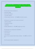
Equilibrium condition:
Actual expenditure = Planned expenditure
Y = PE
“What the economy produces” = “ What the economy plans to produce”
When actual expenditure > planned expenditure -> firms
cannot sell everything they are producing, inventories are
building off, governments and household spend more than
planned -> Firms will reduce their production level, lay of
workers, households and governments will spend less until
you reach the equilibrium situation, until Y falls to
equilibrium level
When the planned expenditure > actual expenditure -> firms
have more demand than the amount they are producing,
households and governments spend les than planned -> firms
produce more, hire more workers, households and
governments will spend less until you reach equilibrium.
, 5. Fiscal policy in the Keynesian cross
G -> Planned expenditure goes up -> unplanned drop in inventory -> firms increase output, hire more workers toward a new equilibrium.
There is a multiplier effect ->
T -> Planned expenditure goes down -> unplanned increase in inventory -> firms decrease
output, lay off workers toward a new equilibrium
There is a tax multiplier
Tax multiplier is negative: A
tax increase reduces C, which reduces income
Is greater than one if MPC (how much you spend if the disposable income
increases) > 0.5: A change in taxes has a multiplier effect in income.
Is smaller than the government spending multiplier: consumers save the
fraction (1- MPC) of a tax cut, so the initial boost in spending from a tax cut is
smaller than from an equal increase in G.
The sum of the government multiplier and the tax multiplier must always be
zero.
6. IS curve
Definition: a graph of all combinations of r and Y that result in goods
market equilibrium.
Actual expenditure (output) = planned expenditure.
Equation -> Y = C( Y – T) + I(r) + G
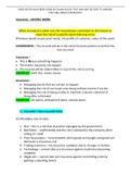
In the Keynesian cross -> I is exogenous but in the IS curve -> I depends
negatively on interest rate.
IS curve slopes downwards -> an increase in the interest rate lowers
investment.
Panel a shows the investment function: an increase in the interest rate
reduces planned investment (reduces investment). Panel b shows the
Keynesian cross -> decrease in planned investment shifts it downwards - >
income reduces from Y1 to Y2. Panel c shows the IS curve summarizing this relationship between interest rate and income. The higher the interest
rate, the lower the level of income.
7. How fiscal policy shifts the IS curve
We can use the IS-LM model to see how fiscal policy (G and T) affects aggregate demand and output -> use the Keynesian cross to see how fiscal
policy shifts the IS curve.
An increase in the government purchases shifts the IS curve outward. In panel a, there is an increase in G -> raises planned expenditure -> increase
in income -> the IS curve shifts right by this amount.
At any value of r, G -> PE -> Y -> IS curve shifts to the right -> horizontal distance of the IS shift equals ->
The IS curve shows the combinations of the interest rate and income that are consistent with equilibrium in the market of goods and services.
Changes in fiscal policy that raise demand for goods shifts IS curve to the right and changes in fiscal policy that reduces the demand for goods
shifts the IS curve to the left.
8. The money market and the LM curve
The LM curve plots the relationship between income and the interest rate that arises in the market for
money balances. Model: Theory of liquidity preference. Due to John Maynard Keynes, A simple theory in
which the interest rate is determined by money supply and money demand
9. Theory of money liquidity
The supply of real money balances is fixed: (M/P)S = M/P
Chapter 10: Introduction to Economic Fluctuations
1. Introduction
Various economic events and policies have different effects over different time horizons.
In the Long run, prices are flexible, responding to changes in supply or demand Classical economic theory: the economy’s output depend on its
ability to supply goods and services, which in turn depends on the supplies of capital and labour and on the available production technology.
In the short run, prices are “sticky” at a predetermined level. The economy behaves much differently when prices are sticky -> e.g. impact of
reduction in money supply Output also depends on the economy’s demand for goods and services. Demand, in turn, depends on many factors:
consumers’ confidence about economic prospects, firms’ perceptions about profitability of new investments, and monetary and fiscal policy.
Economic models illustrate the relationship among the variables.
GDP -> It is the market value of all final goods and services produced within an economy in a given period of time. Sale of used goods is not
included in GDP, changes in inventory don’t change the GDP (e.g. car produced in 2020 but not sold -> affects 2020 GDP but not its consumption,
In 2021 car is sold: C= +20 000, change in inventory: - 20 000 -> GDP hasn’t changed), we don’t count intermediate goods only final goods to avoid
double counting, use the market value and price of each output at its market price and add up the outputs (goods that aren’t sold in the market,
aren’t included in the GDP)
2. Economic fluctuations
Economic fluctuations present a recurring problem for economists and policymakers. Fluctuations in output are closely related with fluctuations in
employment. There is a recession when the economy experiences a period of falling output and rising unemployment. Fluctuations are not regular
and predictable -> what causes fluctuations? Can policymakers avoid recessions?
Short run fluctuations in output -> business cycle.
Model of aggregate supply and demand is used to explain fluctuations.
Starting date of each recession: business cycle peak, ending date: business cycle trough. Recession is a result of at least 2 quarters of declining real
GDP. When economy is in recessions, households respond to fall in their income by consuming less.
Unemployment rises in each recession -> during economic downturns, jobs are harder to find. Increase in unemployment rate -> decrease in real
GDP -> negative relation between unemployment and GDP is called Okun’s Law.
o Percentage change in real GDP -> 3% - 2 x Change in Unemployment Rate (if unemployment rate does not change, real GDP grows by
about 3% but if the unemployment rate rises from 5 to 7%, GDP would fall by 1%.
o Decline in production of goods and services that occur during recessions are always associated with increases in joblessness.
Forecasting because the economic environment affect the governments and the government can use monetary and fiscal policy to affect
economic activity. To forecast, economist look at leading indicators (= variables that often fluctuate before we see movements in the overall
economy).
Average weekly hours in manufacturing (longer workweek = strong demand -> firms increase hiring and production, shorter workweek =
weak demand -> firms lay off workers).
Average weekly claims for unemployment insurance, Manufacturers’ orders for consumer goods and materials and for nondefense
capital goods (increase in orders depletes inventories and increases in production and employment)
ISM new orders index, Index of stock prices, Leading credit index, Interest rate spread, average consumer expectations for business and
economic conditions.
3. Aggregate demand
Aggregate demand relationship between the quantity of output demanded and the aggregate price level.
MV = PY -> M is money supply, V is velocity of money, P is price level, Y is amount of output.
If V is constant then the money supply determines the nominal value of output.
Can be rewritten in terms of supply and demand for real money: M/P = (M/P) d = kY
k = 1/V -> how much money people want to hold for each dollar of income.
Aggregate demand curve slopes downwards -> the money Supply M and velocity of Money V determine the nominal value of output PY. If P goes
up, Y must go down if the price level rises, each transaction requires more dollars so the number of transactions and quantity of goods/ services
purchased must fall.
Shifts in aggregate demand curve -> Ad tells us the possible combinations of P and Y for a given value of M. if the ECB changes the money supply,
then the possible combinations of P and Y change -> Ad curve shifts.
Reduction in money supply shift Ad to the left -> for any given price level the Y is lower, increases in money supply shift the Ad to the right -> for
any given price level the Y is higher.
4. Aggregate supply
, Aggregate supply relationship between the quantity of goods/services supplies and the price level. Aggregate supply depends on the time
horizon. We have two different As: the LRAS and The SRAS.
Long run: vertical aggregate supply curve -> output does not depend on price level, output is determined by the amounts of capital and labour and
technology. The intersection of Ad with the vertical As determines price level.
Y = natural level of output.
Short run: horizontal aggregate supply curve because prices are sticky. The short run equilibrium of the economy Is the intersection of Ad and the
horizontal As -> a fall in aggregate demand reduces output because prices do not adjust instantly.
5. Stabilization policy
Policy actions aimed at reducing the severity of short-run economic fluctuations. Monetary policy is an important component of stabilization
policy.
Shocks to aggregate demand -> an decrease in aggregate demand (people get pessimistic of the economy) -> Y (recession), P (deflation) -> in
the long run, the economy will sell-adjust until Y = YN
Shocks to aggregate supply -> if the price of imported oil goes up -> cost of production -> As shifts up -> Y (recession), P (inflation) -> solved
in 2 ways: laissez faire -> high cyclical unemployment, nominal wages , As shifts down -> Economy self-adjusts or policy makers can shift Ad right
(by M or G or T ) -> Y to YN but P
Chapter 11: Aggregate demand -> building the IS-LM Model
,1. Context of the lecture
Long run: prices flexible, output determined by factors of production and technology, unemployment equals its natural rate.
Short run: prices fixed, output determined by aggregate demand, unemployment negatively related to output
The classical model was incapable of explaining the great depression (unemployment rate was 25%, GDP was less than normal rate), in this model
the GDP depends on factor supplies and available technology -> after depression new model was needed such a large and sudden downturn ->
Keynes proposed a new way to analyse the economy, he proposed that
low aggregate demand is responsible for the low income and high unemployment that characterize economic downturn. He criticized the classical
model for assuming that aggregate supply alone- capital, labour and technology determines national income.
Government can influence aggregate demand with both monetary and fiscal policy.
The IS-LM model was developed by John R. Hicks in the 1930s as an interpretation of John Maynard Keynes’ seminal work, “the General Theory of
Employment, Interest, and Money”. The goal of the model is to show what determines the national income for a given price level
IS: equilibrium in the goods market → IS curve: Investment and Saving.
LM: equilibrium in the money market → LM curve: Liquidity and Money.
Interest rate is the variable that links two halves of the IS-LM model. The model shows how interactions between goods and money markets
determine the position and slope of aggregate demand curve and therefore, the level of national income in the short run.
2. Keynesian model
In the Keynesian economics, the key idea = aggregate demand and they favour activist monetary and fiscal policy to restore aggregate demand
AD = C + I + G + NX -> determines how much flow of expenditure or AD there is to sustain labour hires in a given period.
Nominal wages are sticky -> if the flow of aggregate demand expenditure slows down because wages cannot be cut, workers will have to be laid
off -> lowers the flow of aggregate demand expression.
Problems: Keynesian Model doesn’t always explain why the aggregate demand fell in the first place. Keynesian economics predict that you either
have high unemployment or high inflation but not at the same time -> In America 1970 there was a stagflation -> a lot of economists turned away
from Keynesian ways of thinking.
3. The goods market and the IS curve
The IS curve plots the relationship between income and the interest rate that arises in the market for goods and
services.
4. Keynesian Cross
Keynes proposed that an economy’s total income is, in the short run, determined largely by the
spending plans of households, businesses, and government. The more people want to spend, the more
goods and services firms can sell. The more firms can sell, the more output they will produce and the
more workers they will hire.
Keynes believed that the problem during recessions and depressions is inadequate spending. The
Keynesian cross models this insight.
Distinction between 2 types of expenditures
o Actual expenditure = The amount households, firms and the government spend on goods and services = real GDP = Y
o Planned expenditure = The amount households, firms and the government would like the spend on goods and services -> PE = C + I + G +
NX. In a closed economy -> PE = C + I + G with C = C (Y – T), I = I, G = G, T = T => PE = C( Y – T) + I + G (exogenous variables, is given,
outside of the model). Slope = upward -> when there is more income, people spend more
o Actual and planned expenditure can differ -> Firms can have unplanned inventory
investment when their sales do not meet their expectations.
Equilibrium condition:
Actual expenditure = Planned expenditure
Y = PE
“What the economy produces” = “ What the economy plans to produce”
When actual expenditure > planned expenditure -> firms
cannot sell everything they are producing, inventories are
building off, governments and household spend more than
planned -> Firms will reduce their production level, lay of
workers, households and governments will spend less until
you reach the equilibrium situation, until Y falls to
equilibrium level
When the planned expenditure > actual expenditure -> firms
have more demand than the amount they are producing,
households and governments spend les than planned -> firms
produce more, hire more workers, households and
governments will spend less until you reach equilibrium.
, 5. Fiscal policy in the Keynesian cross
G -> Planned expenditure goes up -> unplanned drop in inventory -> firms increase output, hire more workers toward a new equilibrium.
There is a multiplier effect ->
T -> Planned expenditure goes down -> unplanned increase in inventory -> firms decrease
output, lay off workers toward a new equilibrium
There is a tax multiplier
Tax multiplier is negative: A
tax increase reduces C, which reduces income
Is greater than one if MPC (how much you spend if the disposable income
increases) > 0.5: A change in taxes has a multiplier effect in income.
Is smaller than the government spending multiplier: consumers save the
fraction (1- MPC) of a tax cut, so the initial boost in spending from a tax cut is
smaller than from an equal increase in G.
The sum of the government multiplier and the tax multiplier must always be
zero.
6. IS curve
Definition: a graph of all combinations of r and Y that result in goods
market equilibrium.
Actual expenditure (output) = planned expenditure.
Equation -> Y = C( Y – T) + I(r) + G
In the Keynesian cross -> I is exogenous but in the IS curve -> I depends
negatively on interest rate.
IS curve slopes downwards -> an increase in the interest rate lowers
investment.
Panel a shows the investment function: an increase in the interest rate
reduces planned investment (reduces investment). Panel b shows the
Keynesian cross -> decrease in planned investment shifts it downwards - >
income reduces from Y1 to Y2. Panel c shows the IS curve summarizing this relationship between interest rate and income. The higher the interest
rate, the lower the level of income.
7. How fiscal policy shifts the IS curve
We can use the IS-LM model to see how fiscal policy (G and T) affects aggregate demand and output -> use the Keynesian cross to see how fiscal
policy shifts the IS curve.
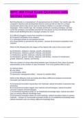
An increase in the government purchases shifts the IS curve outward. In panel a, there is an increase in G -> raises planned expenditure -> increase
in income -> the IS curve shifts right by this amount.
At any value of r, G -> PE -> Y -> IS curve shifts to the right -> horizontal distance of the IS shift equals ->
The IS curve shows the combinations of the interest rate and income that are consistent with equilibrium in the market of goods and services.
Changes in fiscal policy that raise demand for goods shifts IS curve to the right and changes in fiscal policy that reduces the demand for goods
shifts the IS curve to the left.
8. The money market and the LM curve
The LM curve plots the relationship between income and the interest rate that arises in the market for
money balances. Model: Theory of liquidity preference. Due to John Maynard Keynes, A simple theory in
which the interest rate is determined by money supply and money demand
9. Theory of money liquidity
The supply of real money balances is fixed: (M/P)S = M/P