10.1: Various Tests: Introduction
In this module, we will consider various tests that were not covered in previous modules. We will consider
goodness of fit tests, which determines whether or not a statistical model properly describes a set of
observations. In addition, we will look at tests for independence that will tell us whether or not two
variables are related. Finally, we consider ANOVA (analysis of variance) to test whether or not three or
more population means are the same.
Before we study these tests, we must familiarize ourselves with some new distributions (the chi-square
distribution and the F distribution) and learn some basic calculations for multinomial experiments. These
new skills will be attained by studying the pages that follow.
10.2: Chi-Square Distribution
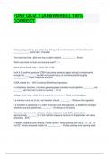
In this module, we will make use of the chi-square distribution. We should consider some of the
characteristics of that distribution. The shape of the chi-square distribution depends on the degrees of
freedom. The chi-square distribution is not symmetric but skewed right. However, as the degrees of
freedom increases, this distribution gets closer and closer to being symmetric. All of the values of this
distribution are non-negative. The total area under the chi-square distribution is equal to 1. The associated
random variable is represented by X2.
Figure 10.1
Values for the chi-square distribution are found using the degrees of freedom (DOF) and the areas in
the right tail of the curve. A chi-square distribution table has been supplied with this course.
Example 10.1. Find the value of X2 for 9 degrees of freedom and an area of .05 in the right tail of the chi-
square distribution.
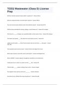
Solution. Please refer to the chi-square distribution table that has been supplied with this course. A
snippet of the table is shown below. Look across the top of the chi-square distribution table for .05
(actually look for X2.05), then look down the left column for 9. The correct value of X 2 is shown in bold.
, Table 10.1: Part of a Chi-square Distribution Table
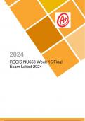
As can be seen in the table above, X2 =16.919. The following figure illustrates the relationship between
the area and X2.
Figure 10.2: Figure for Example 10.1
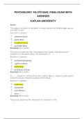
Example 10.2. Find the value of X2 for 17 degrees of freedom and an area of .95 in the right tail of the chi-
square distribution.
Solution. Look across the top of the chi-square distribution table for .95 (actually look for X 2,95), then look
down the left column for 17. These two meet at X2 = 8.672.
Figure 10.3: Figure for Example 10.2
Example 10.3. Find the value of X2 for 30 degrees of freedom and an area of .975 in the left tail of the chi-
square distribution.
Solution. Since the chi-square distribution table gives the area in the right tail of the curve, we must use 1
- .975 = .025. Look across the top of the chi-square distribution table for .025, then look down the left
column for 30. These two meet at X2 = 46.979.
In this module, we will consider various tests that were not covered in previous modules. We will consider
goodness of fit tests, which determines whether or not a statistical model properly describes a set of
observations. In addition, we will look at tests for independence that will tell us whether or not two
variables are related. Finally, we consider ANOVA (analysis of variance) to test whether or not three or
more population means are the same.
Before we study these tests, we must familiarize ourselves with some new distributions (the chi-square
distribution and the F distribution) and learn some basic calculations for multinomial experiments. These
new skills will be attained by studying the pages that follow.
10.2: Chi-Square Distribution
In this module, we will make use of the chi-square distribution. We should consider some of the
characteristics of that distribution. The shape of the chi-square distribution depends on the degrees of
freedom. The chi-square distribution is not symmetric but skewed right. However, as the degrees of
freedom increases, this distribution gets closer and closer to being symmetric. All of the values of this
distribution are non-negative. The total area under the chi-square distribution is equal to 1. The associated
random variable is represented by X2.
Figure 10.1
Values for the chi-square distribution are found using the degrees of freedom (DOF) and the areas in
the right tail of the curve. A chi-square distribution table has been supplied with this course.
Example 10.1. Find the value of X2 for 9 degrees of freedom and an area of .05 in the right tail of the chi-
square distribution.
Solution. Please refer to the chi-square distribution table that has been supplied with this course. A
snippet of the table is shown below. Look across the top of the chi-square distribution table for .05
(actually look for X2.05), then look down the left column for 9. The correct value of X 2 is shown in bold.
, Table 10.1: Part of a Chi-square Distribution Table
As can be seen in the table above, X2 =16.919. The following figure illustrates the relationship between
the area and X2.
Figure 10.2: Figure for Example 10.1
Example 10.2. Find the value of X2 for 17 degrees of freedom and an area of .95 in the right tail of the chi-
square distribution.
Solution. Look across the top of the chi-square distribution table for .95 (actually look for X 2,95), then look
down the left column for 17. These two meet at X2 = 8.672.
Figure 10.3: Figure for Example 10.2
Example 10.3. Find the value of X2 for 30 degrees of freedom and an area of .975 in the left tail of the chi-
square distribution.
Solution. Since the chi-square distribution table gives the area in the right tail of the curve, we must use 1
- .975 = .025. Look across the top of the chi-square distribution table for .025, then look down the left
column for 30. These two meet at X2 = 46.979.