Econometrics Notes 2020-2021
WEEK 1:
Econometrics = using data to measure causal effects.
Univariate analysis: summarizing one variable
Bivariate analysis: summarizing the relationship between 2 variables
Example of a Research question:
*Note: the alternative hypothesis is based on economic theory
What is the random variable and the population?
Numerically summarize the random variable: univariate analysis
Analyze the relationship between the random variable and another random variable: bivariate analysis and
regression analysis
Random variable X = a variable that takes on different values (these are denoted xi) with a given probability for each
outcome [Pr (X = xi)].
In our example, the r.v. is starting salaries of econ grads.
Discrete r.v.: countable outcomes
Continuous r.v.: non-countable outcomes
Population: set of all possible outcomes of X. We think of populations as infinitely large.
In our example, the population is all possible starting salaries of economics graduates
Probability density function (pdf) = function containing the probabilities of different outcomes,
denoted f (xi) = Pr(X = xi).
Discrete pdf: pdf for countable outcomes; (e.g. die rolls)
Continuous pdf: pdf for non-countable outcomes (e.g. hourly wage)
Univariate analysis: numerically summarizing the random variables population pdf
First moment of the pdf: expected value (mean) of X
Second moment of the pdf: variance of X
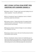
, Variance of the random variable X:
Var (X) = E(X2) - [ E(X) ]2
Bivariate analysis:
We now start considering the relationship between the random variable X and another random variable G:
X= starting salary of econ grads.
G=dummy variable for gender:
o G = 0 for male econ grad
o G = 1 for female econ grad.
To do this, we need the concepts of: joint, marginal and conditional distributions.
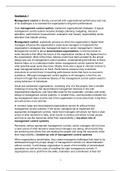
, Joint & marginal distribution
WEEK 1:
Econometrics = using data to measure causal effects.
Univariate analysis: summarizing one variable
Bivariate analysis: summarizing the relationship between 2 variables
Example of a Research question:
*Note: the alternative hypothesis is based on economic theory
What is the random variable and the population?
Numerically summarize the random variable: univariate analysis
Analyze the relationship between the random variable and another random variable: bivariate analysis and
regression analysis
Random variable X = a variable that takes on different values (these are denoted xi) with a given probability for each
outcome [Pr (X = xi)].
In our example, the r.v. is starting salaries of econ grads.
Discrete r.v.: countable outcomes
Continuous r.v.: non-countable outcomes
Population: set of all possible outcomes of X. We think of populations as infinitely large.
In our example, the population is all possible starting salaries of economics graduates
Probability density function (pdf) = function containing the probabilities of different outcomes,
denoted f (xi) = Pr(X = xi).
Discrete pdf: pdf for countable outcomes; (e.g. die rolls)
Continuous pdf: pdf for non-countable outcomes (e.g. hourly wage)
Univariate analysis: numerically summarizing the random variables population pdf
First moment of the pdf: expected value (mean) of X
Second moment of the pdf: variance of X
, Variance of the random variable X:
Var (X) = E(X2) - [ E(X) ]2
Bivariate analysis:
We now start considering the relationship between the random variable X and another random variable G:
X= starting salary of econ grads.
G=dummy variable for gender:
o G = 0 for male econ grad
o G = 1 for female econ grad.
To do this, we need the concepts of: joint, marginal and conditional distributions.
, Joint & marginal distribution