Practical 1
ASSIGNMENT 2 DESCRIPTIVE STAT
The data file contains data about a study on - you guessed it - stress.
More precisely, it contains data on the following variables:
STRESS: Indicates the source of stress, if the participant experiences stress
SMOKE: Indicates if the participant smokes
RELATION: Indicates if the participant is involved in a long-term romantic relationship
OPTIM: Measures how optimistic the participant is on a scale of 0 to 50
SATIS: Measures the life satisfaction of the participant on a scale of 0 to 50
NEGEMO: Measures the amount of negative emotions the participant experiences on a
scale of 0 to 50
Name: Short variable name
● Label: Variable name as displayed in output
● Values: The meaning of the values
● Measure: The level of measurement
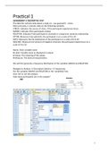
We will first generate a frequency distribution of the variables SMOKE and RELATION.
Navigate to Analyze → Descriptive Statistics → Frequencies.
Put the variables SMOKE and RELATION in the 'variable(s)' box.
Click 'Ok' to run the analysis.
How many participants are in the sample?
780
1
,Question 2: 51.9% of the people in this sample is a smoker.
Question 3: 47.9% of the people in this sample is in a relationship.
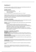
We will now create a histogram of the variable SATIS.
Navigate to Graphs → Legacy Dialogs → Histogram
Make sure to check the box 'Display Normal Curve'.
Click 'Ok' to run the analysis.
The output will now show you a histogram with a superimposed normal curve (i.e. the line
on the histogram).
Can we conclude that the data is normally distributed? YES
Question 4: We could say the data in this histogram are normally distributed, because the
histogram follows the normal curve (the line in the graph) pretty well.
Question 5:
Estimated mean: 26.81 Estimated SD: 6.99
2
,Next up is to generate a table with descriptive statistics.
Navigate to Analyze → Descriptive Statistics → Descriptives
Add the variable SATIS and OPTIM to the 'Variable(s)' box.
Click on “Options” and check the box “Variance”.
Click 'Ok' to run the analysis.
3
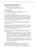
, Besides getting an overall impression of the data, another reason to look at the descriptive
statistics is to see if there are any errors in the data file, such as answers that are outside
the range of expected values.
To find these, you can sort the data file by a variable.
Navigate to Data → Sort Cases
Put the variable OPTIM in the 'Sort by' box.
If you find a strange value, you may select the whole row and delete it.
How many cases did you delete?
OPTIM: Measures how optimistic the participant is on a scale of 0 to 50
SORT CASES BY OPTIM(D).
You should have to delete 1 case, because it has a value for optimism that’s way out of the
range of this variable.
4
ASSIGNMENT 2 DESCRIPTIVE STAT
The data file contains data about a study on - you guessed it - stress.
More precisely, it contains data on the following variables:
STRESS: Indicates the source of stress, if the participant experiences stress
SMOKE: Indicates if the participant smokes
RELATION: Indicates if the participant is involved in a long-term romantic relationship
OPTIM: Measures how optimistic the participant is on a scale of 0 to 50
SATIS: Measures the life satisfaction of the participant on a scale of 0 to 50
NEGEMO: Measures the amount of negative emotions the participant experiences on a
scale of 0 to 50
Name: Short variable name
● Label: Variable name as displayed in output
● Values: The meaning of the values
● Measure: The level of measurement
We will first generate a frequency distribution of the variables SMOKE and RELATION.
Navigate to Analyze → Descriptive Statistics → Frequencies.
Put the variables SMOKE and RELATION in the 'variable(s)' box.
Click 'Ok' to run the analysis.
How many participants are in the sample?
780
1
,Question 2: 51.9% of the people in this sample is a smoker.
Question 3: 47.9% of the people in this sample is in a relationship.
We will now create a histogram of the variable SATIS.
Navigate to Graphs → Legacy Dialogs → Histogram
Make sure to check the box 'Display Normal Curve'.
Click 'Ok' to run the analysis.
The output will now show you a histogram with a superimposed normal curve (i.e. the line
on the histogram).
Can we conclude that the data is normally distributed? YES
Question 4: We could say the data in this histogram are normally distributed, because the
histogram follows the normal curve (the line in the graph) pretty well.
Question 5:
Estimated mean: 26.81 Estimated SD: 6.99
2
,Next up is to generate a table with descriptive statistics.
Navigate to Analyze → Descriptive Statistics → Descriptives
Add the variable SATIS and OPTIM to the 'Variable(s)' box.
Click on “Options” and check the box “Variance”.
Click 'Ok' to run the analysis.
3
, Besides getting an overall impression of the data, another reason to look at the descriptive
statistics is to see if there are any errors in the data file, such as answers that are outside
the range of expected values.
To find these, you can sort the data file by a variable.
Navigate to Data → Sort Cases
Put the variable OPTIM in the 'Sort by' box.
If you find a strange value, you may select the whole row and delete it.
How many cases did you delete?
OPTIM: Measures how optimistic the participant is on a scale of 0 to 50
SORT CASES BY OPTIM(D).
You should have to delete 1 case, because it has a value for optimism that’s way out of the
range of this variable.
4