1
EXERCISE 8 SUGGESTED SOLUTION
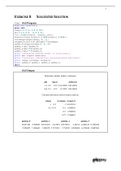
1.(a) SAS Program
goptions reset=all;
proc iml;
omega={1 0.5, 0.5 0.75};
phi={1.2 0.5, -0.6 0.3};
call eigen(eigval, eigvec, phi);
modroots=sqrt(eigval[,1]##2+eigval[,2]##2);
vecomega=shape(omega, 4, 1);
vecgam_0=inv(i(4)-phi@phi)*vecomega;
gamma_0=shape(vecgam_0, 2, 2);
gamma_1=phi*gamma_0;
gamma_2=phi**2*gamma_0;
gamma_3=phi**3*gamma_0;
print 'Determine whether model is stationary';
print phi eigval modroots;
print 'Calculate theoretical autocovariance matrices';
print omega vecomega vecgam_0;
print gamma_0 gamma_1 gamma_2 gamma_3;
quit;
SAS Output
Determine whether model is stationary
phi eigval modroots
1.2 0.5 0.75 0.3122499 0.8124038
-0.6 0.3 0.75 -0.31225 0.8124038
Calculate theoretical autocovariance matrices
omega vecomega vecgam_0
1 0.5 1 10.015183
0.5 0.75 0.5 -5.996952
0.5 -5.996952
0.75 7.1586467
gamma_0 gamma_1 gamma_2 gamma_3
10.015183 -5.996952 9.0197436 -3.617019 6.9195947 -1.46754 4.4263612 0.1859224
-5.996952 7.1586467 -7.808195 5.7457651 -7.754305 3.8939408 -6.478048 2.0487063
WST321
, 2
1 .2 0 .5
Φ =
− 0 .6 0 .3
1.2 − λ 0.5
Φ − λI =
− 0.6 0.3 − λ
= (1.2 − λ )(0.3 − λ ) − (0.5)(−0.6)
= λ2 − 1.5λ + 0.66
=0
The eigenvalues are
λ1 = 0.75 + 0.3122499 i
and
λ2 = 0.75 − 0.31225i .
The modulus of each eigenvalue is
λ1 = (0.75) 2 + (0.3122499) 2
= 0.8124038
and
λ2 = (0.75) 2 + ( −0.31225)2
= 0.8124038 .
Since the modulus for each eigenvalue is less than one, the model is stationary.
The theoretical covariance matrix, Γ0 , is calculated using
vec (Γ 0 ) = [I − (Φ ⊗ Φ)]−1 vec (Ω)
−1
1 0 0 0 1.2 0.5 1.2 0.5 1
1.2 0.5
0 1 0 0 − 0.6 0.3 − 0.6 0.3 0.5
= − 0.5
0 0 1 0 1.2 0.5 1.2 0.5
− 0.6 0.3
0 0 0 1 − 0.6 0.3 − 0.6 0.3 0.75
10.015183
− 5.996952
= .
− 5.996952
7.1586467
WST321
, 3
Therefore
10.015183 − 5.996952
Γ0 = .
− 5.996952 7.1586467
The theoretical autocovariance matrices at lags 1, 2 and 3 are
Γ1 = ΦΓ0
1.2 0.5 10.015183 − 5.996952
=
− 0.6 0.3 − 5.996952 7.1586467
9.0197436 − 3.617019
= ,
− 7.808195 5.7457651
Γ 2 = Φ2 Γ 0
2
1.2 0.5 10.015183 − 5.996952
=
− 0.6 0.3 − 5.996952 7.1586467
6.9195947 − 1.46754
=
− 7.754305 3.8939408
and
Γ3 = Φ3Γ0
3
1.2 0.5 10.015183 − 5.996952
=
− 0.6 0.3 − 5.996952 7.1586467
4.4263612 0.1859224
= .
− 6.478048 2.0487063
WST321
EXERCISE 8 SUGGESTED SOLUTION
1.(a) SAS Program
goptions reset=all;
proc iml;
omega={1 0.5, 0.5 0.75};
phi={1.2 0.5, -0.6 0.3};
call eigen(eigval, eigvec, phi);
modroots=sqrt(eigval[,1]##2+eigval[,2]##2);
vecomega=shape(omega, 4, 1);
vecgam_0=inv(i(4)-phi@phi)*vecomega;
gamma_0=shape(vecgam_0, 2, 2);
gamma_1=phi*gamma_0;
gamma_2=phi**2*gamma_0;
gamma_3=phi**3*gamma_0;
print 'Determine whether model is stationary';
print phi eigval modroots;
print 'Calculate theoretical autocovariance matrices';
print omega vecomega vecgam_0;
print gamma_0 gamma_1 gamma_2 gamma_3;
quit;
SAS Output
Determine whether model is stationary
phi eigval modroots
1.2 0.5 0.75 0.3122499 0.8124038
-0.6 0.3 0.75 -0.31225 0.8124038
Calculate theoretical autocovariance matrices
omega vecomega vecgam_0
1 0.5 1 10.015183
0.5 0.75 0.5 -5.996952
0.5 -5.996952
0.75 7.1586467
gamma_0 gamma_1 gamma_2 gamma_3
10.015183 -5.996952 9.0197436 -3.617019 6.9195947 -1.46754 4.4263612 0.1859224
-5.996952 7.1586467 -7.808195 5.7457651 -7.754305 3.8939408 -6.478048 2.0487063
WST321
, 2
1 .2 0 .5
Φ =
− 0 .6 0 .3
1.2 − λ 0.5
Φ − λI =
− 0.6 0.3 − λ
= (1.2 − λ )(0.3 − λ ) − (0.5)(−0.6)
= λ2 − 1.5λ + 0.66
=0
The eigenvalues are
λ1 = 0.75 + 0.3122499 i
and
λ2 = 0.75 − 0.31225i .
The modulus of each eigenvalue is
λ1 = (0.75) 2 + (0.3122499) 2
= 0.8124038
and
λ2 = (0.75) 2 + ( −0.31225)2
= 0.8124038 .
Since the modulus for each eigenvalue is less than one, the model is stationary.
The theoretical covariance matrix, Γ0 , is calculated using
vec (Γ 0 ) = [I − (Φ ⊗ Φ)]−1 vec (Ω)
−1
1 0 0 0 1.2 0.5 1.2 0.5 1
1.2 0.5
0 1 0 0 − 0.6 0.3 − 0.6 0.3 0.5
= − 0.5
0 0 1 0 1.2 0.5 1.2 0.5
− 0.6 0.3
0 0 0 1 − 0.6 0.3 − 0.6 0.3 0.75
10.015183
− 5.996952
= .
− 5.996952
7.1586467
WST321
, 3
Therefore
10.015183 − 5.996952
Γ0 = .
− 5.996952 7.1586467
The theoretical autocovariance matrices at lags 1, 2 and 3 are
Γ1 = ΦΓ0
1.2 0.5 10.015183 − 5.996952
=
− 0.6 0.3 − 5.996952 7.1586467
9.0197436 − 3.617019
= ,
− 7.808195 5.7457651
Γ 2 = Φ2 Γ 0
2
1.2 0.5 10.015183 − 5.996952
=
− 0.6 0.3 − 5.996952 7.1586467
6.9195947 − 1.46754
=
− 7.754305 3.8939408
and
Γ3 = Φ3Γ0
3
1.2 0.5 10.015183 − 5.996952
=
− 0.6 0.3 − 5.996952 7.1586467
4.4263612 0.1859224
= .
− 6.478048 2.0487063
WST321