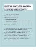
Macroeconomics: Output and Time
Factor IS LM FE AD AS DAD SAS
Equilibriu Aggregate Money BoP = 0 IS = LM = Labour IS = LM = Labour supply
m economy = demand CA + CP = FE supply FE, = Labour
aggregate (Ld) = 0 = adjusted to demand,
expenditure Money CA = -CP Labour inflation adjusted to
supply demand inflation
(goods (m) (foreign
market) exchange (labour
(money market) market)
market)
Shape Downward Upward Horizona Downward Short Downward Upward
sloping sloping l sloping run: sloping sloping
Upward
sloping;
(Long
run:
vertical)
Shifters Shifts to the Shifts to Shifts up All IS-LM- Shifts to All AD All AS
right if: the if: FE shifters the shifters, shifters,
G↑ right if: Iworld ↑ (Fixed: IS right if: adjusted adjusted for
R↑ M↑ and W↑ for inflation
Yworld
↑ Flexible: P ↓ inflation
I↑ LM and
EX ↑ FE)
P world
↑
IM ↓
T↓
Space i–Y i–Y i–Y P–Y P–Y π–Y π–Y
1−c 1+G k 1 i=i¿
world
Fixed: e
p= p +(Y −Y ) ¿
Flex: π=π e + λ ( Y −Y ¿ )
i= Y + i= Y − M
b b h h p=m−bY +h(i world + ε e ) π=μ−bY +b Y t −1+ h ( ∆ i w + ∆ ε e )
Flex: Fixed:
world world
p=e+ p + δG+ γ Y π=ε −f (i+world
w
π −bY+ϵ e )+ bY t−1 +γ ∆ Y w +δ ∆G−
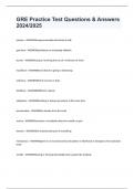
→ Mundell-Fleming model (IS-LM-FE): useful for understanding short-run movements
(demand-side)
Does a policy affect output Y?
Fixed exchange rate system Flexible exchange rate
Fiscal policy by Government Yes No
Spending (G) or Taxes (T) (full crowding out via
exchange rate)
Monetary policy by Money No Yes
Supply (M) (forced sterilization through
intervention)
1
, → Under flexible exchange rates the positions of FE and LM are set exogenously (set by
policymakers). The exchange rate determines the position of IS, and endogenously adjusts to
let IS pass through the given point of intersection between FE an LM.
→ Under fixed exchange rates, the positions of FE and IS are set exogenously. The money
supply, which determines the position of LM, endogenously adjusts to let LM pass through
the given point of intersection between FE and IS.
Exchange rate
Nominal exchange rate (E)
Real exchange rate (R) = E*(Pworld/P)
o Depreciation – R ↑ → good for EX, bad for IM
o Appreciation – R ↓ → good for IM, bad for EX
Balance of Payments = detailed record of international transactions (exports and imports).
Three main components:
1) Current account (CA) – records the cross border transactions → EX – IM
o Vertical line (CA = 0, when balanced)
o To the left from CA = 0 → CA surplus; To the right from CA = 0 → CA deficit
o Line shifts left if R ↓ or Yworld ↓; opposite for shift to the right
2) Capital account (CP) – purchases and sales of foreign assets that do not involve CB
(net transfer of assets and liabilities)
o Horizontal line (i=i world ) → under perfect capital mobility with k → ∞ ;
Under perfect immobility (full capital controls/no capital flows), the FE
curve becomes independent of iworld and turns vertical
o i<i world → investors will invest in other countries and CP < 0
o i>i world → investors will invest in the country and CP > 0
3) Official reserve account (OR) – Central Bank actions on FE market (assumed 0 with
fully feasible (CB not involved) exchange rate)
→ BoP = CA + CP + OR = 0
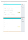
Potential output (equilibrium output) defines what economy produced if it leaves no
available factors of production idle. Main two factors that affect the production potential of
a country are: capital (K) and labour (L). → Y = F(K, L), also known as the production function
MPL is the slope of the partial production function and measures how much output is gained
by a small increase of labour → shows decreasing marginal returns; MPL goes down the
more workers you add after a certain threshold
Labour determination
o Firms will continue to hire more workers until it is no longer profitable for them →
when real wage (w) = W/P equals extra revenue (MPL). w = MPL (profit line) is the
most profitable → when w > MPL: unprofitable territory
How can we explain unemployment at equilibrium? (1) Tax wedge; (2) Minimum wage
→ Real wage rigidity is a market imperfection that keeps the real wage from falling to the
level that eliminates involuntary employment.
2
Factor IS LM FE AD AS DAD SAS
Equilibriu Aggregate Money BoP = 0 IS = LM = Labour IS = LM = Labour supply
m economy = demand CA + CP = FE supply FE, = Labour
aggregate (Ld) = 0 = adjusted to demand,
expenditure Money CA = -CP Labour inflation adjusted to
supply demand inflation
(goods (m) (foreign
market) exchange (labour
(money market) market)
market)
Shape Downward Upward Horizona Downward Short Downward Upward
sloping sloping l sloping run: sloping sloping
Upward
sloping;
(Long
run:
vertical)
Shifters Shifts to the Shifts to Shifts up All IS-LM- Shifts to All AD All AS
right if: the if: FE shifters the shifters, shifters,
G↑ right if: Iworld ↑ (Fixed: IS right if: adjusted adjusted for
R↑ M↑ and W↑ for inflation
Yworld
↑ Flexible: P ↓ inflation
I↑ LM and
EX ↑ FE)
P world
↑
IM ↓
T↓
Space i–Y i–Y i–Y P–Y P–Y π–Y π–Y
1−c 1+G k 1 i=i¿
world
Fixed: e
p= p +(Y −Y ) ¿
Flex: π=π e + λ ( Y −Y ¿ )
i= Y + i= Y − M
b b h h p=m−bY +h(i world + ε e ) π=μ−bY +b Y t −1+ h ( ∆ i w + ∆ ε e )
Flex: Fixed:
world world
p=e+ p + δG+ γ Y π=ε −f (i+world
w
π −bY+ϵ e )+ bY t−1 +γ ∆ Y w +δ ∆G−
→ Mundell-Fleming model (IS-LM-FE): useful for understanding short-run movements
(demand-side)
Does a policy affect output Y?
Fixed exchange rate system Flexible exchange rate
Fiscal policy by Government Yes No
Spending (G) or Taxes (T) (full crowding out via
exchange rate)
Monetary policy by Money No Yes
Supply (M) (forced sterilization through
intervention)
1
, → Under flexible exchange rates the positions of FE and LM are set exogenously (set by
policymakers). The exchange rate determines the position of IS, and endogenously adjusts to
let IS pass through the given point of intersection between FE an LM.
→ Under fixed exchange rates, the positions of FE and IS are set exogenously. The money
supply, which determines the position of LM, endogenously adjusts to let LM pass through
the given point of intersection between FE and IS.
Exchange rate
Nominal exchange rate (E)
Real exchange rate (R) = E*(Pworld/P)
o Depreciation – R ↑ → good for EX, bad for IM
o Appreciation – R ↓ → good for IM, bad for EX
Balance of Payments = detailed record of international transactions (exports and imports).
Three main components:
1) Current account (CA) – records the cross border transactions → EX – IM
o Vertical line (CA = 0, when balanced)
o To the left from CA = 0 → CA surplus; To the right from CA = 0 → CA deficit
o Line shifts left if R ↓ or Yworld ↓; opposite for shift to the right
2) Capital account (CP) – purchases and sales of foreign assets that do not involve CB
(net transfer of assets and liabilities)
o Horizontal line (i=i world ) → under perfect capital mobility with k → ∞ ;
Under perfect immobility (full capital controls/no capital flows), the FE
curve becomes independent of iworld and turns vertical
o i<i world → investors will invest in other countries and CP < 0
o i>i world → investors will invest in the country and CP > 0
3) Official reserve account (OR) – Central Bank actions on FE market (assumed 0 with
fully feasible (CB not involved) exchange rate)
→ BoP = CA + CP + OR = 0
Potential output (equilibrium output) defines what economy produced if it leaves no
available factors of production idle. Main two factors that affect the production potential of
a country are: capital (K) and labour (L). → Y = F(K, L), also known as the production function
MPL is the slope of the partial production function and measures how much output is gained
by a small increase of labour → shows decreasing marginal returns; MPL goes down the
more workers you add after a certain threshold
Labour determination
o Firms will continue to hire more workers until it is no longer profitable for them →
when real wage (w) = W/P equals extra revenue (MPL). w = MPL (profit line) is the
most profitable → when w > MPL: unprofitable territory
How can we explain unemployment at equilibrium? (1) Tax wedge; (2) Minimum wage
→ Real wage rigidity is a market imperfection that keeps the real wage from falling to the
level that eliminates involuntary employment.
2