Operations Management
Week 1
Operations Management= the set of activities that creates value in the form of goods and
services by transforming inputs into outputs.
1. Performance requirements and analysis
2. Process design
3. Planning and scheduling
Productivity
Productivity= a way of measuring process improvement. It represents the output of a
process relative to its inputs.
Single factor productivity= Units produced/Input used
Multi factor productivity= Output/(Labor + Material + Energy + Capital + Miscellaneous)
Learning Curves
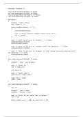
Learning curves= time needed to produce a
unit decreases with each additional unit.
The decrease in time follows an exponential
curve called learning or experience curve.
A learning rate of L, means that each time
the production doubles, the time needed for
producing a unit will equal the original
production time multiplied by L.
Suppose that students learn at a rate of
L=0.60 (or 60%). It took students 25
minutes to solve the exercise.
It takes 0.6*25= 15 minutes for the second exercise and 0.6*0.6*25= 9 minutes for the
fourth exercise and 0.6*0.6*0.6*25= 5.4 minutes for the eighth exercise.
Logarithmic approach when the values do not double:
Tn= T1 * N^(log L/log 2) N=unit of interest T1= time needed for unit 1
A shipyard wants to sell 17 ships to a customer. Calculate the minimum learning rate if
the 17th ship cannot take more time than 65 days to build, assuming the rst ship will
take a 100 days.
65= 100 * 17^(log L/log2) —> L=0.90
Queuing Models
Using the queuing theory, we can nd estimates for how
certain systems will perform. Decision problem: balance cost
of providing good service with cost of customers waiting.
fi fi
, Poisson distribution= number of events that occur in an interval of time. Customer arrivals
are independent.
Negative exponential distribution= the service time and time between arrivals.
Types of queuing models:
1. Simple (M/M/1), poisson distribution arrivals, negatively distributed service times, 1
server, e.g. information booth at a mall.
2. Multi-channel (M/M/S), poisson distribution arrivals, negatively distributed service
times, multiple service, e.g. airline ticket counter.
3. Constant Service (M/D/1), poisson distribution arrivals, service time is the same, 1
server, e.g. automated car wash.
Example
A co ee-corner in a large mall is sta ed by one employee. On average 60 customers
arrive per hour (Poisson arrivals). It takes on average 20 seconds to serve a fresh cup of
co ee (negative exponential service times). What is the average time a customer has to
wait before they can start drinking co ee?
M/M/1 model λ= 60 customers/hour μ= 180 customers/hour
The time a customer has to wait is the time spent in the queue and the serving time= Ws.
Ws= 1/ (μ - λ)
Ws= 1/ (180-60)= 0.0083 hours
Performance Measures
Utilisation rate (M/M/1) or M/D/1): p= λ/μ
Utilisation rate (M/M/S): p= λ/(Sμ)
Probability of 0 units in the system/system idle:
P0= 1- λ /μ
Probability of having more than k units in the system:
P n>k = (λ / μ)^(k+1) n=number of units in the system
Little’s Law= describes the relationship between the number of people in the system and
the waiting time in the system. If you know the arrival rate and waiting time in the system
you can calculate the number of units in the system. Ls= λ * Ws and Lq= λ * Wq.
Relationship between Wq/Lq and Ws/Ls= the average time spent in the queue equals the
average time spent in the system minus the average time spent in the server. Therefore,
Wq= Ws - 1/μ. The average number of units in the queue equals the average number of
units in the system minus the average number of units in the server, Lq= Ls - λ/μ
Week 2
Deterministic Performance Estimation
Performance analysis= compare estimated performance of proposals.
ff ff ffff
, Di erences in simulation studies and deterministic estimates of performance are caused
by: in deterministic performance estimation we assume there is no uncertainty. In a
simulation model we can imitate variability.
Flow diagram= schematic drawing of the movement of material, product or people.
Normal distribution= describes the uncertainty around the mean.
Throughput time
Throughput time= time that passes between the moment at which the product is taken
into production and the moment at which the product is ready. Deterministic throughput
time can be estimated by adding the cycle times of the di erent operations. Deterministic
means that you ignore any probability distributions and just use the average value. We
ignore waiting line e ects. Ws is thus the time a product spends in the system.
Deterministic throughput time= 6 + 2 + 4= 12 minutes
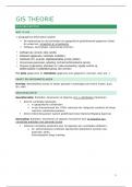
Throughput time with multiple paths
Red (upper) route:
6 + 2 + 4= 12 minutes
Blue (lower) route:
6 + 2 + 12= 20 minutes
Total= 0.6 x 12 + 0.40 x 20= 15.2
minutes
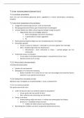
Design capacity= theoretical
maximum output of a system or
process in a given period.
E ective capacity= capacity that
can be expected given the product
mix, methods of scheduling,
maintenance and standards of quality.
Serial processing (steps are performed consecutively)
ffff
ff ff
Week 1
Operations Management= the set of activities that creates value in the form of goods and
services by transforming inputs into outputs.
1. Performance requirements and analysis
2. Process design
3. Planning and scheduling
Productivity
Productivity= a way of measuring process improvement. It represents the output of a
process relative to its inputs.
Single factor productivity= Units produced/Input used
Multi factor productivity= Output/(Labor + Material + Energy + Capital + Miscellaneous)
Learning Curves
Learning curves= time needed to produce a
unit decreases with each additional unit.
The decrease in time follows an exponential
curve called learning or experience curve.
A learning rate of L, means that each time
the production doubles, the time needed for
producing a unit will equal the original
production time multiplied by L.
Suppose that students learn at a rate of
L=0.60 (or 60%). It took students 25
minutes to solve the exercise.
It takes 0.6*25= 15 minutes for the second exercise and 0.6*0.6*25= 9 minutes for the
fourth exercise and 0.6*0.6*0.6*25= 5.4 minutes for the eighth exercise.
Logarithmic approach when the values do not double:
Tn= T1 * N^(log L/log 2) N=unit of interest T1= time needed for unit 1
A shipyard wants to sell 17 ships to a customer. Calculate the minimum learning rate if
the 17th ship cannot take more time than 65 days to build, assuming the rst ship will
take a 100 days.
65= 100 * 17^(log L/log2) —> L=0.90
Queuing Models
Using the queuing theory, we can nd estimates for how
certain systems will perform. Decision problem: balance cost
of providing good service with cost of customers waiting.
fi fi
, Poisson distribution= number of events that occur in an interval of time. Customer arrivals
are independent.
Negative exponential distribution= the service time and time between arrivals.
Types of queuing models:
1. Simple (M/M/1), poisson distribution arrivals, negatively distributed service times, 1
server, e.g. information booth at a mall.
2. Multi-channel (M/M/S), poisson distribution arrivals, negatively distributed service
times, multiple service, e.g. airline ticket counter.
3. Constant Service (M/D/1), poisson distribution arrivals, service time is the same, 1
server, e.g. automated car wash.
Example
A co ee-corner in a large mall is sta ed by one employee. On average 60 customers
arrive per hour (Poisson arrivals). It takes on average 20 seconds to serve a fresh cup of
co ee (negative exponential service times). What is the average time a customer has to
wait before they can start drinking co ee?
M/M/1 model λ= 60 customers/hour μ= 180 customers/hour
The time a customer has to wait is the time spent in the queue and the serving time= Ws.
Ws= 1/ (μ - λ)
Ws= 1/ (180-60)= 0.0083 hours
Performance Measures
Utilisation rate (M/M/1) or M/D/1): p= λ/μ
Utilisation rate (M/M/S): p= λ/(Sμ)
Probability of 0 units in the system/system idle:
P0= 1- λ /μ
Probability of having more than k units in the system:
P n>k = (λ / μ)^(k+1) n=number of units in the system
Little’s Law= describes the relationship between the number of people in the system and
the waiting time in the system. If you know the arrival rate and waiting time in the system
you can calculate the number of units in the system. Ls= λ * Ws and Lq= λ * Wq.
Relationship between Wq/Lq and Ws/Ls= the average time spent in the queue equals the
average time spent in the system minus the average time spent in the server. Therefore,
Wq= Ws - 1/μ. The average number of units in the queue equals the average number of
units in the system minus the average number of units in the server, Lq= Ls - λ/μ
Week 2
Deterministic Performance Estimation
Performance analysis= compare estimated performance of proposals.
ff ff ffff
, Di erences in simulation studies and deterministic estimates of performance are caused
by: in deterministic performance estimation we assume there is no uncertainty. In a
simulation model we can imitate variability.
Flow diagram= schematic drawing of the movement of material, product or people.
Normal distribution= describes the uncertainty around the mean.
Throughput time
Throughput time= time that passes between the moment at which the product is taken
into production and the moment at which the product is ready. Deterministic throughput
time can be estimated by adding the cycle times of the di erent operations. Deterministic
means that you ignore any probability distributions and just use the average value. We
ignore waiting line e ects. Ws is thus the time a product spends in the system.
Deterministic throughput time= 6 + 2 + 4= 12 minutes
Throughput time with multiple paths
Red (upper) route:
6 + 2 + 4= 12 minutes
Blue (lower) route:
6 + 2 + 12= 20 minutes
Total= 0.6 x 12 + 0.40 x 20= 15.2
minutes
Design capacity= theoretical
maximum output of a system or
process in a given period.
E ective capacity= capacity that
can be expected given the product
mix, methods of scheduling,
maintenance and standards of quality.
Serial processing (steps are performed consecutively)
ffff
ff ff