CHAPTER 1
Economic Models
A. Summary
This chapter provides an introduction to the book by showing why
economists use simplified models. The chapter begins with a few
definitions of economics and then turns to a discussion of such
models. Development of Marshall's analysis of supply and demand is
the principle example used here, and this provides a review for
students of what they learned in introductory economics. The notion
of how shifts in supply or demand curves affect equilibrium prices is
highlighted and is repeated in the chapter’s appendix in a somewhat
more formal way. The chapter also reminds students of the
production possibility frontier concept and shows how it illustrates
opportunity costs. The chapter concludes with a discussion of how
economic models might be verified. A brief description of the
distinction between positive and normative analysis is also presented.
B. Lecture and Discussion Suggestions
We have found that a useful way to start the course is with one (or
perhaps two) lectures on the historical development of microeconomics
together with some current examples. For example, many students find
economic applications to the natural world fascinating and some of the
economics behind Application 1.1, might be examined. The simple
model of the world oil market in Application 1A.3 is also a good way to
introduce models with real world numbers in them. Application 1.6:
Economic Confusion provides normative distinction and to tell a few
economic jokes (several Internet sites offer such jokes if your supply is
running low).
C. Glossary Entries in the Chapter
• Diminishing Returns
• Economics
• Equilibrium Price
• Microeconomics
• Models
, • Opportunity Cost
• Positive Normative Distinction
• Production Possibility Frontier
• Supply-Demand Model
• Testing Assumptions
• Testing Predictions
APPENDIX TO CHAPTER 1
Mathematics Used in
Microeconomics
A. Summary
This appendix provides a review of basic algebra with a specific
focus on the graphical tools that students will encounter later in the
text. The coverage of linear and quadratic equations here is quite
standard and should be familiar to students. Two concepts that will
be new to some students are graphing contour lines and
simultaneous equations. The discussion of contour lines seeks to
introduce students to the indifference curve concept through the
contour map analogy. Although students may not have graphed such
a family of curves for a many-variable function before, this
introduction seems to provide good preparation for the economic
applications that follow.
The analysis of simultaneous equations presented in the appendix
is intended to illustrate how the solution to two linear equations in
two unknowns is reflected graphically by the intersection of the two
lines. Although students may be familiar with solving simultaneous
equations through substitution or subtraction, this graphical approach
may not be so well known. Because such graphic solutions lead
directly to the economic concept of supply-demand equilibrium,
however, I believe it is useful to introduce this method of solution to
students. Showing how a shift in one of the equations changes the
solutions for both variables is particularly instructive in that regard.
In that regard, some material at the end of the appendix makes the
, distinction between endogenous and exogenous variables – a
distinction that many students stumble over.
The appendix also contains a few illustrations of calculus-type
results. Depending on student preparation, instructors might wish
to pick up on this and use a few calculus ideas in later chapters. But
this is not a calculus-based text, so there is no need to do this.
B. Lecture and Discussion Suggestions
Since much of the material in this appendix is self-explanatory, most
instructors may prefer to skip any lecture on this topic. For those
who feel a lecture is useful, we would suggest developing a specific
numerical example together with graphic and tabular handouts for
students. The presentation should, focus primarily on linear
equations since these are most widely used in the book and since
students will be most familiar with them.
C. Glossary Entries in the Chapter
• Average Effect
• Contour Lines
• Dependent Variable
• Functional Notation
• Independent Variable
• Intercept
• Linear Function
• Marginal Effect
• Simultaneous Equations
• Slope
• Statistical Inference
• Variables
SOLUTIONS TO CHAPTER 1 PROBLEMS
, 1.1 a.
b. Yes, the points seem to be on straight lines. For the demand curve: P
=1
Q = –100
Q
P=a−
100
at P = 1, Q = 700, so a = 8 and
Q
P =8− or Q = 800 − 100 P
100
For the supply curve, the points also seem to be on a straight line:
P 1
=
Q 200
Q
If P = a + bQ = a +
200
Economic Models
A. Summary
This chapter provides an introduction to the book by showing why
economists use simplified models. The chapter begins with a few
definitions of economics and then turns to a discussion of such
models. Development of Marshall's analysis of supply and demand is
the principle example used here, and this provides a review for
students of what they learned in introductory economics. The notion
of how shifts in supply or demand curves affect equilibrium prices is
highlighted and is repeated in the chapter’s appendix in a somewhat
more formal way. The chapter also reminds students of the
production possibility frontier concept and shows how it illustrates
opportunity costs. The chapter concludes with a discussion of how
economic models might be verified. A brief description of the
distinction between positive and normative analysis is also presented.
B. Lecture and Discussion Suggestions
We have found that a useful way to start the course is with one (or
perhaps two) lectures on the historical development of microeconomics
together with some current examples. For example, many students find
economic applications to the natural world fascinating and some of the
economics behind Application 1.1, might be examined. The simple
model of the world oil market in Application 1A.3 is also a good way to
introduce models with real world numbers in them. Application 1.6:
Economic Confusion provides normative distinction and to tell a few
economic jokes (several Internet sites offer such jokes if your supply is
running low).
C. Glossary Entries in the Chapter
• Diminishing Returns
• Economics
• Equilibrium Price
• Microeconomics
• Models
, • Opportunity Cost
• Positive Normative Distinction
• Production Possibility Frontier
• Supply-Demand Model
• Testing Assumptions
• Testing Predictions
APPENDIX TO CHAPTER 1
Mathematics Used in
Microeconomics
A. Summary
This appendix provides a review of basic algebra with a specific
focus on the graphical tools that students will encounter later in the
text. The coverage of linear and quadratic equations here is quite
standard and should be familiar to students. Two concepts that will
be new to some students are graphing contour lines and
simultaneous equations. The discussion of contour lines seeks to
introduce students to the indifference curve concept through the
contour map analogy. Although students may not have graphed such
a family of curves for a many-variable function before, this
introduction seems to provide good preparation for the economic
applications that follow.
The analysis of simultaneous equations presented in the appendix
is intended to illustrate how the solution to two linear equations in
two unknowns is reflected graphically by the intersection of the two
lines. Although students may be familiar with solving simultaneous
equations through substitution or subtraction, this graphical approach
may not be so well known. Because such graphic solutions lead
directly to the economic concept of supply-demand equilibrium,
however, I believe it is useful to introduce this method of solution to
students. Showing how a shift in one of the equations changes the
solutions for both variables is particularly instructive in that regard.
In that regard, some material at the end of the appendix makes the
, distinction between endogenous and exogenous variables – a
distinction that many students stumble over.
The appendix also contains a few illustrations of calculus-type
results. Depending on student preparation, instructors might wish
to pick up on this and use a few calculus ideas in later chapters. But
this is not a calculus-based text, so there is no need to do this.
B. Lecture and Discussion Suggestions
Since much of the material in this appendix is self-explanatory, most
instructors may prefer to skip any lecture on this topic. For those
who feel a lecture is useful, we would suggest developing a specific
numerical example together with graphic and tabular handouts for
students. The presentation should, focus primarily on linear
equations since these are most widely used in the book and since
students will be most familiar with them.
C. Glossary Entries in the Chapter
• Average Effect
• Contour Lines
• Dependent Variable
• Functional Notation
• Independent Variable
• Intercept
• Linear Function
• Marginal Effect
• Simultaneous Equations
• Slope
• Statistical Inference
• Variables
SOLUTIONS TO CHAPTER 1 PROBLEMS
, 1.1 a.
b. Yes, the points seem to be on straight lines. For the demand curve: P
=1
Q = –100
Q
P=a−
100
at P = 1, Q = 700, so a = 8 and
Q
P =8− or Q = 800 − 100 P
100
For the supply curve, the points also seem to be on a straight line:
P 1
=
Q 200
Q
If P = a + bQ = a +
200