Genetics in Neuroscience – exam 1
Statistical Refresher
Random variable
variable that varies over subjects, cases, participants, etc.
For example sex, weight, height, IQ, neuroticism, eye color, alcohol consumption, etc.
Environmental: urban vs. rural.
Genetic: ABO blood group genotype.
yi = b0 + b1 · xi + 𝜀i
The yi and xi are observed and the 𝜀i is unobserved.
If we know b0 and b1 exactly, then 𝜀I could be observed. However, b0 and b1 are estimates and we can
never know them exactly, so 𝜀I is always unobserved.
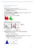
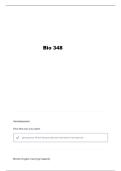
The distribution of a RV is a histogram.
Discrete: sex, eye color, hair color, pregnancy, depression.
Binomial Uniform
Continuous: testosterone level, BMI, intelligence, depression.
Can have a normal distribution.
0 = normal
N De 1 = depressed
0
1
Continuous Discrete
Interval – linear regression Ordinal – logistic regression
Normal distribution: characterized by two parameters mean and standard deviation.
Mean: average value of a sample.
or sum (p(value) · #value)
SD: measure of spread, dispersion or variation.
Variance: SD²; provides a quantitative measure of individual differences. This is what we want
to explain in behavioral genetics!
The larger, the greater the magnitude of individual differences.
or sum ( (value – mean)² · p(value) )
1
,Association between variables
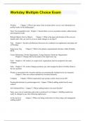
linear relationship between continuous random variables.
We want to know the joint (bivariate) distribution of X and Y do X and Y co-vary?
Covariance: scale dependent, so hard to interpret.
Correlation: standardized measure r.
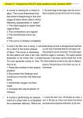
The stronger the relationship, the more straight the regression line is.
r = 0.00 r = 0.40 r = 0.90
Covariance matrix: symmetric by definition, because the covariance between X and Y equals the
covariance between Y and X. It is a characteristic of the population.
X Y X Y
X sx² sXY X 10 4
Y sXY sY² Y 4 13
Correlation matrix: the SD = √𝑠²
SDX = sX = √10 = 3.16
SDY = sY = √13 = 3.61
Correlation = covariance / (SDX ·SDY)
We can standardize the covariance matrix and get the correlation matrix:
X Y X Y
X sx² / (sX · sX) sXY / (sX . sY) X 10 / (3.16 · 3.16) 4 / (3.16 · 3.61)
Y sXY / (sX . sY) sY² / (sY . sY) Y 4 / (3.16 · 3.61) 13 / (3.61 · 3.61)
The correlation matrix is equal to the X Y
covariance between z-scores of the X 1 0.35
variables. Y 0.35 1
𝑥−𝑚𝑒𝑎𝑛
z = 𝑆𝐷
IQ raw scores IQ z-scores
Mean = 100.53 Mean = 0
SD = 15.36 SD =1
Var = 235.95 Var =1
Linear regression analysis
yi = b0 + b1 · xi + 𝜀i
b0 is the intercept; expected (predicted) value of Y if X=0.
b1 is the slope / regression coefficient; expresses the strength of the linear relationship.
How much Y is expected to change given a unit change in X.
𝜀i is the residual / prediction error; discrepancy between Y-predicted and Y-observed.
sY² = b1² · sX² + sE²
Explained and not explained
R² is the proportion of variance of Y that is explained by the predictor X effect size.
The explained variance of Y / total variance of Y
b1² · sX² b1² · sX²
R² = 𝑠𝑌² = b1² · sX² + sE² is equal to standardized β if you have 1 predictor.
The correlation coefficient r r² = R² so r = R
H0: b1 = 0 / R² = 0
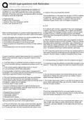
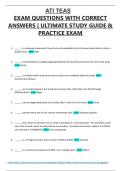
Distributional assumption: assumption of homoscedasticity.
The residual of Y given any value of X is normally distributed with a mean of 0 and variance of s E²
2
,Don’t make any assumption about the distribution of predictor X or outcome Y!
It’s a conditional distribution: Y | X is normally distributed.
A binary X variable is not normally distributed by definition!
A binary Y variable (discrete) means that there can’t be linear regression possible, so the distributional
assumption can’t be verified!
Mean(Y) = b0 + b1 · mean(X)
Variance(Y) = b1² · variance(X) + variance(ε)
R² = b1² · var(X) / b1² · var(X) + var(ε)
= explained var / total variance
Estimate Std. Error t value Pr(>|t|)
b 6.4000 1.5476 4.135 7.49e-05 ***
0
b 0.4000 0.1079 3.709 0.000345 ***
1
Multiple R-squared: 0.1231
p<0.05, so H0 is rejected and t-value is too large given H0
b1 also characterizes the joint distribution of X and Y covariance matrix
X Y
X 10 4
Y 4 13
Mean 14 12
var(Y) = explained + not explained
X Y
X var(X) b1 · var(X)
Y b1 · var(X) b1² · var(X) + var(ε)
Mean mean(X) b0 + b1 · mean(X)
X Y
X 10 0.4 · 10 = 4
Y 0.4 · 10 = 4 0.4² · 10 + 11.4 = 13
Mean 14 6.4 + 0.4 · 14 = 12
R² = (0.4² · 10) / (0.4² · 10 + 11.4)
R² = 1.6 / (1.6+11.4)
R² = 0.123
So, 12.3% of the variance of Y is “explained”
3
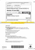
, Possible outcomes of statistical analysis:
Truth
b1 = 0 b1 ≠ 0
Decision b1 = 0 1-α β (type II error)
b1 ≠ 0 α (type I error) 1-β
Type I error rate: the chance of making a wrong decision 0.05
Power: 1-β; probability of (correctly) deciding that the effect is present (b 1 ≠ 0) while in truth the effect
is present (b1 ≠ 0).
Test statistic: deciding to reject H0 if the test statistic is too extreme.
𝑏1
t = 𝑆𝐸
df = N-parameters (are b0 and b1)
Probabilities
Throw dice 100 times N=100 p( X | Y ) = p( X and Y ) / p(Y)
1 2 3 4 5 6 p( X and Y ) = p(X) · p(Y)
# 15 14 19 15 11 26
p 0.15 0.14 0.19 0.15 0.11 0.26 Eye color can be light (L) or dark (D).
Unconditional p(outcome=1) = = 0.15 Hair color can be fair/red (FR), medium (M)
and black/dark (BD).
Conditional p(outcome=1 | outcome<4) FR M BD
N of outcome 1/2/3 = 15+14+19 = 48 L 1168 825 305 2298
p(outcome=1 | outcome<4) = = 0.3125 D 573 1312 1200 3085
1 2 3 1741 2137 1505 5383
# 15 14 19 N=5383
Unconditional p 0.15 0.14 0.19 p = #outcome / total
Observed 0.3125 0.2916 0.3958 FR M BD
conditional p L 0.22 0.15 0.06 0.43
Expected 0.3333 0.3333 0.3333 D 0.11 0.24 0.22 0.57
conditional p 0.32 0.40 0.28 1
Conditional probability:
Odds(event) = p / (1-p)
p( FR | L) = p( FR and L) / p(L)
If the chance (p) of the event = 0.5
p( FR | L) = 0..43 = 0.51
Odds = 0.5 / (1-0.5) = 1
p( FR | L) = = 0.51
p = odds / (1+odds)
Unconditional probability:
If the odds are 1
p(FR) = = 0.32
p = 1 / (1+1) = 0.5
p(L) = = 0.43
Odds ratio = odds(A) / odds(B)
p( FR or M ) = (1741+2137) / 5383 = 0.72
= (pA / 1-pA) / (pB / 1-pB)
Relative risk: probability of X given Y1 is …
times the probability of X given Y2
Ratio of conditional probabilities
p( FR | L) = 0..43 = 0.51
p( FR | D) = 0..57 = 0.19
RR = 0..19 = 2.73
Light eyes increase the risk of fair hair relative
to dark eyes.
4
Statistical Refresher
Random variable
variable that varies over subjects, cases, participants, etc.
For example sex, weight, height, IQ, neuroticism, eye color, alcohol consumption, etc.
Environmental: urban vs. rural.
Genetic: ABO blood group genotype.
yi = b0 + b1 · xi + 𝜀i
The yi and xi are observed and the 𝜀i is unobserved.
If we know b0 and b1 exactly, then 𝜀I could be observed. However, b0 and b1 are estimates and we can
never know them exactly, so 𝜀I is always unobserved.
The distribution of a RV is a histogram.
Discrete: sex, eye color, hair color, pregnancy, depression.
Binomial Uniform
Continuous: testosterone level, BMI, intelligence, depression.
Can have a normal distribution.
0 = normal
N De 1 = depressed
0
1
Continuous Discrete
Interval – linear regression Ordinal – logistic regression
Normal distribution: characterized by two parameters mean and standard deviation.
Mean: average value of a sample.
or sum (p(value) · #value)
SD: measure of spread, dispersion or variation.
Variance: SD²; provides a quantitative measure of individual differences. This is what we want
to explain in behavioral genetics!
The larger, the greater the magnitude of individual differences.
or sum ( (value – mean)² · p(value) )
1
,Association between variables
linear relationship between continuous random variables.
We want to know the joint (bivariate) distribution of X and Y do X and Y co-vary?
Covariance: scale dependent, so hard to interpret.
Correlation: standardized measure r.
The stronger the relationship, the more straight the regression line is.
r = 0.00 r = 0.40 r = 0.90
Covariance matrix: symmetric by definition, because the covariance between X and Y equals the
covariance between Y and X. It is a characteristic of the population.
X Y X Y
X sx² sXY X 10 4
Y sXY sY² Y 4 13
Correlation matrix: the SD = √𝑠²
SDX = sX = √10 = 3.16
SDY = sY = √13 = 3.61
Correlation = covariance / (SDX ·SDY)
We can standardize the covariance matrix and get the correlation matrix:
X Y X Y
X sx² / (sX · sX) sXY / (sX . sY) X 10 / (3.16 · 3.16) 4 / (3.16 · 3.61)
Y sXY / (sX . sY) sY² / (sY . sY) Y 4 / (3.16 · 3.61) 13 / (3.61 · 3.61)
The correlation matrix is equal to the X Y
covariance between z-scores of the X 1 0.35
variables. Y 0.35 1
𝑥−𝑚𝑒𝑎𝑛
z = 𝑆𝐷
IQ raw scores IQ z-scores
Mean = 100.53 Mean = 0
SD = 15.36 SD =1
Var = 235.95 Var =1
Linear regression analysis
yi = b0 + b1 · xi + 𝜀i
b0 is the intercept; expected (predicted) value of Y if X=0.
b1 is the slope / regression coefficient; expresses the strength of the linear relationship.
How much Y is expected to change given a unit change in X.
𝜀i is the residual / prediction error; discrepancy between Y-predicted and Y-observed.
sY² = b1² · sX² + sE²
Explained and not explained
R² is the proportion of variance of Y that is explained by the predictor X effect size.
The explained variance of Y / total variance of Y
b1² · sX² b1² · sX²
R² = 𝑠𝑌² = b1² · sX² + sE² is equal to standardized β if you have 1 predictor.
The correlation coefficient r r² = R² so r = R
H0: b1 = 0 / R² = 0
Distributional assumption: assumption of homoscedasticity.
The residual of Y given any value of X is normally distributed with a mean of 0 and variance of s E²
2
,Don’t make any assumption about the distribution of predictor X or outcome Y!
It’s a conditional distribution: Y | X is normally distributed.
A binary X variable is not normally distributed by definition!
A binary Y variable (discrete) means that there can’t be linear regression possible, so the distributional
assumption can’t be verified!
Mean(Y) = b0 + b1 · mean(X)
Variance(Y) = b1² · variance(X) + variance(ε)
R² = b1² · var(X) / b1² · var(X) + var(ε)
= explained var / total variance
Estimate Std. Error t value Pr(>|t|)
b 6.4000 1.5476 4.135 7.49e-05 ***
0
b 0.4000 0.1079 3.709 0.000345 ***
1
Multiple R-squared: 0.1231
p<0.05, so H0 is rejected and t-value is too large given H0
b1 also characterizes the joint distribution of X and Y covariance matrix
X Y
X 10 4
Y 4 13
Mean 14 12
var(Y) = explained + not explained
X Y
X var(X) b1 · var(X)
Y b1 · var(X) b1² · var(X) + var(ε)
Mean mean(X) b0 + b1 · mean(X)
X Y
X 10 0.4 · 10 = 4
Y 0.4 · 10 = 4 0.4² · 10 + 11.4 = 13
Mean 14 6.4 + 0.4 · 14 = 12
R² = (0.4² · 10) / (0.4² · 10 + 11.4)
R² = 1.6 / (1.6+11.4)
R² = 0.123
So, 12.3% of the variance of Y is “explained”
3
, Possible outcomes of statistical analysis:
Truth
b1 = 0 b1 ≠ 0
Decision b1 = 0 1-α β (type II error)
b1 ≠ 0 α (type I error) 1-β
Type I error rate: the chance of making a wrong decision 0.05
Power: 1-β; probability of (correctly) deciding that the effect is present (b 1 ≠ 0) while in truth the effect
is present (b1 ≠ 0).
Test statistic: deciding to reject H0 if the test statistic is too extreme.
𝑏1
t = 𝑆𝐸
df = N-parameters (are b0 and b1)
Probabilities
Throw dice 100 times N=100 p( X | Y ) = p( X and Y ) / p(Y)
1 2 3 4 5 6 p( X and Y ) = p(X) · p(Y)
# 15 14 19 15 11 26
p 0.15 0.14 0.19 0.15 0.11 0.26 Eye color can be light (L) or dark (D).
Unconditional p(outcome=1) = = 0.15 Hair color can be fair/red (FR), medium (M)
and black/dark (BD).
Conditional p(outcome=1 | outcome<4) FR M BD
N of outcome 1/2/3 = 15+14+19 = 48 L 1168 825 305 2298
p(outcome=1 | outcome<4) = = 0.3125 D 573 1312 1200 3085
1 2 3 1741 2137 1505 5383
# 15 14 19 N=5383
Unconditional p 0.15 0.14 0.19 p = #outcome / total
Observed 0.3125 0.2916 0.3958 FR M BD
conditional p L 0.22 0.15 0.06 0.43
Expected 0.3333 0.3333 0.3333 D 0.11 0.24 0.22 0.57
conditional p 0.32 0.40 0.28 1
Conditional probability:
Odds(event) = p / (1-p)
p( FR | L) = p( FR and L) / p(L)
If the chance (p) of the event = 0.5
p( FR | L) = 0..43 = 0.51
Odds = 0.5 / (1-0.5) = 1
p( FR | L) = = 0.51
p = odds / (1+odds)
Unconditional probability:
If the odds are 1
p(FR) = = 0.32
p = 1 / (1+1) = 0.5
p(L) = = 0.43
Odds ratio = odds(A) / odds(B)
p( FR or M ) = (1741+2137) / 5383 = 0.72
= (pA / 1-pA) / (pB / 1-pB)
Relative risk: probability of X given Y1 is …
times the probability of X given Y2
Ratio of conditional probabilities
p( FR | L) = 0..43 = 0.51
p( FR | D) = 0..57 = 0.19
RR = 0..19 = 2.73
Light eyes increase the risk of fair hair relative
to dark eyes.
4