INFERENTIAL STATISTICS EXAM PART II
Complete study guide sorted per lecture
Based on the studybook Stats: Data and Models, 5th Edition
Richard D. De Veaux & Paul F. Velleman
University of Twente
Block 1B 2021-2022
Lecture 8: non-parametric tests 2
- Chapter 20 (section 4 and 5)
- Chapter 20 (section 22.5 (skip Turkeys Quick test), p 649 + example canvas)
- Chapter 21
Lecture 9: regression: assumptions + using the model 12
- Chapter 23 (section 1 and 3 (page 733, 734, 740 – 744)
- Chapter 23 (section 2 (page 735 – 739. Assumptions and conditions) > 9.1.)
- Chapter 23 (section 6 (page 721-722) > 9.2.)
Lecture 10: introduction to multiple regression 27
- Chapter 9 (section 1, 2 and 3)
- Chapter 23 (section 5)
- Chapter 23 (section 8)
Lecture 11: inference about more than two means 35
- Chapter 26
- Chapter 25 (section 1, 2, 3 and 5)
Lecture 12: inference for two-way ANOVA 62
- Chapter 26
Lecture 13: more about multiple regression and analysis of variance (ANOVA) 78
- Chapter 9
- Chapter 23
Lecture 14: overview, reflection and preparation for the exam 101
1
,Lecture 8: non-parametric tests
23 december 2021
Main objective: knowing how to construct a test for the difference between two means if the assumptions for a
parametric test are not fulfilled. To realize this, we ask the following questions
- How can we investigate normality?
- What can we do when the assumptions for the t-test of two means are not fulfilled?
- When can we use the Wilcoxon rank sum test? + execute it
- When can we use the Wilcoxon signed rank test? + execute it
o When can we use the Kruskal Wallis test? > lecture 11
Read:
- Chapter 20 section 4 till 5
- Chapter 20 section 22.5 (skip Turkeys Quick test), p 649 + example canvas
- Chapter 21
Other content
- Notes lecture
- Chapter 20: exercise 67
- Chapter 21: exercise 27
- Chapter 21: exercise 29
- 8.1. exercise 1
- 8.1. exercise 2
- 8.1. exercise 3
2
,20.4. a confidence interval for the difference between two means.
Imagine: a researcher wants to know if people bid more/less money when they buy a camera from their friends, in
comparison with buying a camera from a stranger. You can find this:
- Mean of bids in the group of buying from friends: 281,88
- Mean of bids in the group of buying from strangers: 211,43
This is from a sample. But how big a difference should we expect in general? Comparing two means is just like
comparing two proportions.
- The parameter of interest is the difference between the two means. Mu1 – mu2.
- The statistic of interest is ybar 1 – ybar 2. We’ll start with this statistic to build a confidence interval and
we’ll use the same standard deviation and sampling distribution as we did for the hypothesis test.
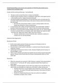
To find “the standard deviation – of the samplings distribution of the difference between the two independent
sample means” we add their variances and then take the square root. So this leads to:
In this notation we use sigma. But ofcourse we don’t know it. So we use the estimates, s1 and s2. Using the
estimates gives us the standard error.
We use the standard error to judge how big the difference really is. Because we are estimating, again we will use
students T model.
The confidence interval we build is called a two-sample t-interval (for the difference in means).
The corresponding hypothesis test is called a two-sample t-test.
The interval looks just like the ones we’ve seen before (the statistics +/- as estimated margin of error)
We are still missing the degrees of freedom we need when using the students T. This formula is strange.
** the deep secret is that the sampling model isn’t really students T, but only something close. The trick is by using
a special degrees of freedom value, we can make it close to students T model. The adjustment formula is
straightforward but doesn’t help our understanding much. The formula is on the bottom of page 641. In the formula
sheet that Harry gave us, its denoted as DF = min (n1-1 : n2-1)
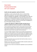
A sampling distribution model for the difference between two means
When conditions are met, the sampling distribution of the standardized sample difference between the means of
two independent groups
Can be modelled by a students t model. With a number of degrees freedom found with a special formula. We
estimate the standard error with
3
, Assumptions and conditions
This test is sometimes called the two independent samples t-test, because it is only appropriate when the responses
of the two groups are independent from each other. No statistical test can verify this assumption. You have to think
about how the data were collected.
- Independence assumption
o Independence condition. Within each group, individual responses should be independent of each
other. Knowing one’s response should provide no information about other responses.
o Randomization condition. If the responses are selected with randomization, their independence
is likely.
o Independent groups assumption: the responses in the two groups we are comparing must also be
independent of each other. Knowing how one group responds should not provide information
about the other group. Usually, the independence of the groups from each other is evident from
the way the data are collected
▪ Violation is for the groups to be paired
o When we have quantitative data: check for outliers, skewness, multiple modes and other
surprises. We check this for each group.
- Normal population assumption. If you are comparing the means of two groups then (as we did before
with students t-models) you must assume that the underlying populations are each Normally distributed.
o Nearly normal condition for both groups. A violation of either one violates the condition. The
bigger the group, the less problematic a slightly skewed histogram is. When both groups are big
enough, the Central Limit Theorem forms an escape.
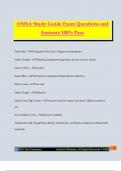
A two-sample t-interval for the difference between means
When the conditions are met, we are ready to find the confidence interval for: the difference between means of
two independent groups (mu1 – mu2). The confidence interval is
Where the standard error is the difference of the means is
The critical value t (t*) depends on the particular confidence level (C) that you specify and on the number of
degrees of freedom, which we get from the sample sized and a special formula. But in this course by Harry’s
formula of DF = min (n1-1 : n2-1)
Questions:
Why is the randomization of the patients into two Randomization should balance unknown sources of
treatments important? variability in the two groups of patients and helps us believe
the two groups are independent
A 95% confidence interval for the difference in We can be 96% confident that after 4 weeks surgery patients
mean strength is about (0,04kg, 2.96kg). Explain will have a mean strength between 0,04 kg and 2,96 kg
what this interval means. higher than non-surgery patients.
Why might we want to examine such a The lower bound of this interval is close to 0, so the
confidence interval in deciding between two difference may not be great enough that patients could
options? actually notice the difference. We want to consider other
issues such as costs and risks in making a recommendation
about the two options.
Why might you want to see the data before Without data we can’t check the nearly normal condition.
trusting the confidence interval?
4
Complete study guide sorted per lecture
Based on the studybook Stats: Data and Models, 5th Edition
Richard D. De Veaux & Paul F. Velleman
University of Twente
Block 1B 2021-2022
Lecture 8: non-parametric tests 2
- Chapter 20 (section 4 and 5)
- Chapter 20 (section 22.5 (skip Turkeys Quick test), p 649 + example canvas)
- Chapter 21
Lecture 9: regression: assumptions + using the model 12
- Chapter 23 (section 1 and 3 (page 733, 734, 740 – 744)
- Chapter 23 (section 2 (page 735 – 739. Assumptions and conditions) > 9.1.)
- Chapter 23 (section 6 (page 721-722) > 9.2.)
Lecture 10: introduction to multiple regression 27
- Chapter 9 (section 1, 2 and 3)
- Chapter 23 (section 5)
- Chapter 23 (section 8)
Lecture 11: inference about more than two means 35
- Chapter 26
- Chapter 25 (section 1, 2, 3 and 5)
Lecture 12: inference for two-way ANOVA 62
- Chapter 26
Lecture 13: more about multiple regression and analysis of variance (ANOVA) 78
- Chapter 9
- Chapter 23
Lecture 14: overview, reflection and preparation for the exam 101
1
,Lecture 8: non-parametric tests
23 december 2021
Main objective: knowing how to construct a test for the difference between two means if the assumptions for a
parametric test are not fulfilled. To realize this, we ask the following questions
- How can we investigate normality?
- What can we do when the assumptions for the t-test of two means are not fulfilled?
- When can we use the Wilcoxon rank sum test? + execute it
- When can we use the Wilcoxon signed rank test? + execute it
o When can we use the Kruskal Wallis test? > lecture 11
Read:
- Chapter 20 section 4 till 5
- Chapter 20 section 22.5 (skip Turkeys Quick test), p 649 + example canvas
- Chapter 21
Other content
- Notes lecture
- Chapter 20: exercise 67
- Chapter 21: exercise 27
- Chapter 21: exercise 29
- 8.1. exercise 1
- 8.1. exercise 2
- 8.1. exercise 3
2
,20.4. a confidence interval for the difference between two means.
Imagine: a researcher wants to know if people bid more/less money when they buy a camera from their friends, in
comparison with buying a camera from a stranger. You can find this:
- Mean of bids in the group of buying from friends: 281,88
- Mean of bids in the group of buying from strangers: 211,43
This is from a sample. But how big a difference should we expect in general? Comparing two means is just like
comparing two proportions.
- The parameter of interest is the difference between the two means. Mu1 – mu2.
- The statistic of interest is ybar 1 – ybar 2. We’ll start with this statistic to build a confidence interval and
we’ll use the same standard deviation and sampling distribution as we did for the hypothesis test.
To find “the standard deviation – of the samplings distribution of the difference between the two independent
sample means” we add their variances and then take the square root. So this leads to:
In this notation we use sigma. But ofcourse we don’t know it. So we use the estimates, s1 and s2. Using the
estimates gives us the standard error.
We use the standard error to judge how big the difference really is. Because we are estimating, again we will use
students T model.
The confidence interval we build is called a two-sample t-interval (for the difference in means).
The corresponding hypothesis test is called a two-sample t-test.
The interval looks just like the ones we’ve seen before (the statistics +/- as estimated margin of error)
We are still missing the degrees of freedom we need when using the students T. This formula is strange.
** the deep secret is that the sampling model isn’t really students T, but only something close. The trick is by using
a special degrees of freedom value, we can make it close to students T model. The adjustment formula is
straightforward but doesn’t help our understanding much. The formula is on the bottom of page 641. In the formula
sheet that Harry gave us, its denoted as DF = min (n1-1 : n2-1)
A sampling distribution model for the difference between two means
When conditions are met, the sampling distribution of the standardized sample difference between the means of
two independent groups
Can be modelled by a students t model. With a number of degrees freedom found with a special formula. We
estimate the standard error with
3
, Assumptions and conditions
This test is sometimes called the two independent samples t-test, because it is only appropriate when the responses
of the two groups are independent from each other. No statistical test can verify this assumption. You have to think
about how the data were collected.
- Independence assumption
o Independence condition. Within each group, individual responses should be independent of each
other. Knowing one’s response should provide no information about other responses.
o Randomization condition. If the responses are selected with randomization, their independence
is likely.
o Independent groups assumption: the responses in the two groups we are comparing must also be
independent of each other. Knowing how one group responds should not provide information
about the other group. Usually, the independence of the groups from each other is evident from
the way the data are collected
▪ Violation is for the groups to be paired
o When we have quantitative data: check for outliers, skewness, multiple modes and other
surprises. We check this for each group.
- Normal population assumption. If you are comparing the means of two groups then (as we did before
with students t-models) you must assume that the underlying populations are each Normally distributed.
o Nearly normal condition for both groups. A violation of either one violates the condition. The
bigger the group, the less problematic a slightly skewed histogram is. When both groups are big
enough, the Central Limit Theorem forms an escape.
A two-sample t-interval for the difference between means
When the conditions are met, we are ready to find the confidence interval for: the difference between means of
two independent groups (mu1 – mu2). The confidence interval is
Where the standard error is the difference of the means is
The critical value t (t*) depends on the particular confidence level (C) that you specify and on the number of
degrees of freedom, which we get from the sample sized and a special formula. But in this course by Harry’s
formula of DF = min (n1-1 : n2-1)
Questions:
Why is the randomization of the patients into two Randomization should balance unknown sources of
treatments important? variability in the two groups of patients and helps us believe
the two groups are independent
A 95% confidence interval for the difference in We can be 96% confident that after 4 weeks surgery patients
mean strength is about (0,04kg, 2.96kg). Explain will have a mean strength between 0,04 kg and 2,96 kg
what this interval means. higher than non-surgery patients.
Why might we want to examine such a The lower bound of this interval is close to 0, so the
confidence interval in deciding between two difference may not be great enough that patients could
options? actually notice the difference. We want to consider other
issues such as costs and risks in making a recommendation
about the two options.
Why might you want to see the data before Without data we can’t check the nearly normal condition.
trusting the confidence interval?
4