Statistical Tests
Chi-squared test
χ² test: comparing proportions between groups.
The frequencies for the levels of nominal/ordinal variables can be presented in a contingency
table.
Assumptions:
Sample is randomly taken from the population assumed under the H0.
No expected frequencies < 1.
No more than 20% expected frequencies < 5.
Observed frequencies: the frequencies observed in the sample.
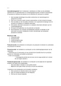
Expected frequencies:
Example blond boy:
marg(a) = total of one group (28)
marg(b) = total of other group (22)
total = total/total (47)
Look up the critical value of under df and α.
If the calculated < critical value not significant, so H0 is not rejected.
If the calculated > critical value significant, so H0 is rejected.
In 2x2 tables, the tends to be too large (p-values too small), so a type I error.
Than it is best to use the Yates correction.
Fisher test? P. 723.
1
, Pearson correlation
Is always between -1 and +1.
What is the association strength between variable x and y?
H0: The correlation coefficient is 0.
H1: The correlation coefficient is different from 0.
Assumptions:
Relation must be linear: can see this by plotting data (x,y).
Variables are bivariate normally distributed: for each value of x, the values of y are
normally distributed.
Homescedasticity of variances: the variance does not depend on score.
Analyze Correlate Bivariate
To test whether r is significantly different from 0, you have to convert the r into a z-score or t
test statistic, since r does not have a normal distribution.
Look up z-score in the table for normal distribution (small portion one-sided p-value).
and
Confidence interval of z-score:
Lower bound: 𝑧𝑟 − (1.96 ∗ 𝑆𝐸𝑧𝑟 )
Upper bound: 𝑧𝑟 + (1.96 ∗ 𝑆𝐸𝑧𝑟 )
𝑒 2𝑧𝑟 −1
Convert back to confidence interval of r: 𝑟 =
𝑒 2𝑧𝑟 +1
Spearman's rank correlation (rho or rs)
Non-parametric variant of Pearson correlation.
Lies between -1 and +1
Rank scores within the variables.
Calculate the difference between ranks.
o When N>30, than:
and
2
Chi-squared test
χ² test: comparing proportions between groups.
The frequencies for the levels of nominal/ordinal variables can be presented in a contingency
table.
Assumptions:
Sample is randomly taken from the population assumed under the H0.
No expected frequencies < 1.
No more than 20% expected frequencies < 5.
Observed frequencies: the frequencies observed in the sample.
Expected frequencies:
Example blond boy:
marg(a) = total of one group (28)
marg(b) = total of other group (22)
total = total/total (47)
Look up the critical value of under df and α.
If the calculated < critical value not significant, so H0 is not rejected.
If the calculated > critical value significant, so H0 is rejected.
In 2x2 tables, the tends to be too large (p-values too small), so a type I error.
Than it is best to use the Yates correction.
Fisher test? P. 723.
1
, Pearson correlation
Is always between -1 and +1.
What is the association strength between variable x and y?
H0: The correlation coefficient is 0.
H1: The correlation coefficient is different from 0.
Assumptions:
Relation must be linear: can see this by plotting data (x,y).
Variables are bivariate normally distributed: for each value of x, the values of y are
normally distributed.
Homescedasticity of variances: the variance does not depend on score.
Analyze Correlate Bivariate
To test whether r is significantly different from 0, you have to convert the r into a z-score or t
test statistic, since r does not have a normal distribution.
Look up z-score in the table for normal distribution (small portion one-sided p-value).
and
Confidence interval of z-score:
Lower bound: 𝑧𝑟 − (1.96 ∗ 𝑆𝐸𝑧𝑟 )
Upper bound: 𝑧𝑟 + (1.96 ∗ 𝑆𝐸𝑧𝑟 )
𝑒 2𝑧𝑟 −1
Convert back to confidence interval of r: 𝑟 =
𝑒 2𝑧𝑟 +1
Spearman's rank correlation (rho or rs)
Non-parametric variant of Pearson correlation.
Lies between -1 and +1
Rank scores within the variables.
Calculate the difference between ranks.
o When N>30, than:
and
2