Samenvatting macroeconomics
The short run
2. Chapter 2: the core introduction
• Nominal GDP = sum of quantities of final goods produce times their current price
o GDP rises over time because production and price of most goods increases over time
• Real GDP = sum of quantities of final goods produced times a constant price
o Constant price instead of current price
o It’s the weighted average of the output of all final goods
• Positive GDP growth = expanion; negative GDP growth = recession
• GDP deflator shows how increases in nominal GDP can come from an increase in prices of in
real GDP
o Pt = nominal GDPt / real GDPt
3. Chapter 3: The goods market
3.1. The composition of gdp
• Y = GDP
• C = Consumption
• I = investments
• G = government spending
• X = exports
• IM = imports
3.2. The demand for goods
• Demand for goods = Z = C + I + G + X - IM
o Assumption: we operate in a closed economy: Z = C + I + G
• Consumption
o Disposable income = the income that remains once consumers have paid taxes and
received transfers from the government
YD = Y – T
• Y = income
o Consumption function:
C = C(YD)
C = c0 + c1(YD)
• C0 = the amount people would consume if their disposable income
would be equal to zero
• C1 = propensity to consume = the effect that an additional euro of
disposable income has on the consumption
C = c0 + c1(Y-T)
1
,• Investment
o Investment is seen as exogenous
Consumtion is endogenous
• Het streepje erboven wilt gewoon zeggen dat we investment nemen
zoals gegeven om het model eenvoudig te houden
• Investment verandert niet bij verandering in productie
• Government spending
o G&T
o Also exogenous
3.3. Determination of equilibrium output
• Z = c0 + c1(Y – T) + I + G
• Production Y = demand for goods Z
• Y = c0 + c1(Y – T) + I + G -> hieruit volgt:
o Bestaat uit 2 delen:
Multiplier = 1/(1-c1)
Autonomous spending = c0 + I + G – c1T
• Graph:
o
En Y = income
o 2 grafieken:
Productie Y ifv. Inkomen Y
Vraag Z ifv. Inkomen Y
o In het equilibrium is de productie Y gelijk aan de vraag Z
2
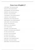
,o Increase in autonomous spendinig on output:
Vraag neemt toe met 1 miljoen
Omdat de vraag is toegenomen zal ook de productie toenemen met 1
miljoen (A->B). Omdat de productie is toegenomen zullen ook de lonen
stijgen (B->C)
De vraag neemt hierdoor opnieuw toe -> productie neemt opnieuw toe (C-
>D) deze keer met c1*1 miljoen -> lonen nemen met dezelfde waarde toe (D-
>E)
3
, Opnieuw wordt deze cyclus doorlopen en verhoogt het met factor
C1²*1miljoen. Dit blijft zo nog een tijdje doorgaan tot het terug in een
stabiele situatie komt waar vraag en productie gelijk zijn
Geen één op één effect, een toename van 1 miljoen in vraag zorgt voor een
veel grotere toename. Deze toename is gelijk aan:
• 1 miljoen * (1+ c1 + c12 + … + c1n)
• = 1 miljoen * 1/(1-c1)
• Onzekerheid -> voorzichtigheid -> saving (c0 daalt)
3.4. Investment equals savings: alternative wayof goods-market equilibrium
• Saving = sum of private and public saving
o S = YD – C
o S=Y-T–C
Private saving = S
Public saving = T – G
• Als T>G: budget surplus
• Als T<G: budget deficit
• Equilibrium in the goods market: IS relation
o Y=C+I+G Y–T–C=I+G–T S=I+G–T
Vgl 2: Substract T from both sides
Vlg 3: Met Y-T = YD en YD-C = S
o I = S + (T – G)
o Equilibrium in the goods market requires that investment equals savings (sum of
private and public savings)
o This is the IS relation
What firms want to invest must be equal to what governments and people
want to save
o S = Y – T – C S = Y – T – c0 – c1(Y - T) S = – c0 + (1 – c1)(Y - T)
o I = -c0 + (1 – c1)(Y - T) + (T - G)
1 – c1 is called the marginal propensity to save
o
3.5. The paradox of saving
• When people attempt to save more, the result is both a decline in output and unchanged
saving
• -> show mathematically: reduce c0
3.6. Is the government omnipotent? A warning
• G & T are considered as exogenous and under control of the government
o Changing government taxes is not always easy
• Responses of consumption, investment, imports etc. are hard to assess with much certainty
• Anticipations are likely to matter
• Achieving a given level of output can come with unpleasant side effects
• Budget deficits and public debt may have adverse implications in the long run
4
The short run
2. Chapter 2: the core introduction
• Nominal GDP = sum of quantities of final goods produce times their current price
o GDP rises over time because production and price of most goods increases over time
• Real GDP = sum of quantities of final goods produced times a constant price
o Constant price instead of current price
o It’s the weighted average of the output of all final goods
• Positive GDP growth = expanion; negative GDP growth = recession
• GDP deflator shows how increases in nominal GDP can come from an increase in prices of in
real GDP
o Pt = nominal GDPt / real GDPt
3. Chapter 3: The goods market
3.1. The composition of gdp
• Y = GDP
• C = Consumption
• I = investments
• G = government spending
• X = exports
• IM = imports
3.2. The demand for goods
• Demand for goods = Z = C + I + G + X - IM
o Assumption: we operate in a closed economy: Z = C + I + G
• Consumption
o Disposable income = the income that remains once consumers have paid taxes and
received transfers from the government
YD = Y – T
• Y = income
o Consumption function:
C = C(YD)
C = c0 + c1(YD)
• C0 = the amount people would consume if their disposable income
would be equal to zero
• C1 = propensity to consume = the effect that an additional euro of
disposable income has on the consumption
C = c0 + c1(Y-T)
1
,• Investment
o Investment is seen as exogenous
Consumtion is endogenous
• Het streepje erboven wilt gewoon zeggen dat we investment nemen
zoals gegeven om het model eenvoudig te houden
• Investment verandert niet bij verandering in productie
• Government spending
o G&T
o Also exogenous
3.3. Determination of equilibrium output
• Z = c0 + c1(Y – T) + I + G
• Production Y = demand for goods Z
• Y = c0 + c1(Y – T) + I + G -> hieruit volgt:
o Bestaat uit 2 delen:
Multiplier = 1/(1-c1)
Autonomous spending = c0 + I + G – c1T
• Graph:
o
En Y = income
o 2 grafieken:
Productie Y ifv. Inkomen Y
Vraag Z ifv. Inkomen Y
o In het equilibrium is de productie Y gelijk aan de vraag Z
2
,o Increase in autonomous spendinig on output:
Vraag neemt toe met 1 miljoen
Omdat de vraag is toegenomen zal ook de productie toenemen met 1
miljoen (A->B). Omdat de productie is toegenomen zullen ook de lonen
stijgen (B->C)
De vraag neemt hierdoor opnieuw toe -> productie neemt opnieuw toe (C-
>D) deze keer met c1*1 miljoen -> lonen nemen met dezelfde waarde toe (D-
>E)
3
, Opnieuw wordt deze cyclus doorlopen en verhoogt het met factor
C1²*1miljoen. Dit blijft zo nog een tijdje doorgaan tot het terug in een
stabiele situatie komt waar vraag en productie gelijk zijn
Geen één op één effect, een toename van 1 miljoen in vraag zorgt voor een
veel grotere toename. Deze toename is gelijk aan:
• 1 miljoen * (1+ c1 + c12 + … + c1n)
• = 1 miljoen * 1/(1-c1)
• Onzekerheid -> voorzichtigheid -> saving (c0 daalt)
3.4. Investment equals savings: alternative wayof goods-market equilibrium
• Saving = sum of private and public saving
o S = YD – C
o S=Y-T–C
Private saving = S
Public saving = T – G
• Als T>G: budget surplus
• Als T<G: budget deficit
• Equilibrium in the goods market: IS relation
o Y=C+I+G Y–T–C=I+G–T S=I+G–T
Vgl 2: Substract T from both sides
Vlg 3: Met Y-T = YD en YD-C = S
o I = S + (T – G)
o Equilibrium in the goods market requires that investment equals savings (sum of
private and public savings)
o This is the IS relation
What firms want to invest must be equal to what governments and people
want to save
o S = Y – T – C S = Y – T – c0 – c1(Y - T) S = – c0 + (1 – c1)(Y - T)
o I = -c0 + (1 – c1)(Y - T) + (T - G)
1 – c1 is called the marginal propensity to save
o
3.5. The paradox of saving
• When people attempt to save more, the result is both a decline in output and unchanged
saving
• -> show mathematically: reduce c0
3.6. Is the government omnipotent? A warning
• G & T are considered as exogenous and under control of the government
o Changing government taxes is not always easy
• Responses of consumption, investment, imports etc. are hard to assess with much certainty
• Anticipations are likely to matter
• Achieving a given level of output can come with unpleasant side effects
• Budget deficits and public debt may have adverse implications in the long run
4