ii
, SOLUTIONS MANUAL
for
An Introduction to
The Finite Element Method
(Third Edition)
by
J. N. REDDY
Department of Mechanical Engineering
Texas A & M University
College Station, Texas 77843-3123
PROPRIETARY AND CONFIDENTIAL
This Manual is the proprietary property of The McGraw-Hill Companies, Inc.
(“McGraw-Hill”) and protected by copyright and other state and federal laws. By
opening and using this Manual the user agrees to the following restrictions, and if
the recipient does not agree to these restrictions, the Manual should be promptly
returned unopened to McGraw-Hill: This Manual is being provided only to
authorized professors and instructors for use in preparing for the classes
using the affiliated textbook. No other use or distribution of this Manual
is permitted. This Manual may not be sold and may not be distributed to
or used by any student or other third party. No part of this Manual
may be reproduced, displayed or distributed in any form or by any
means, electronic or otherwise, without the prior written permission of
the McGraw-Hill.
McGraw-Hill, New York, 2005
, 1
Chapter 1
INTRODUCTION
Problem 1.1: Newton’s second law can be expressed as
F = ma (1)
where F is the net force acting on the body, m mass of the body, and a the
acceleration of the body in the direction of the net force. Use Eq. (1) to determine
the mathematical model, i.e., governing equation of a free-falling body. Consider
only the forces due to gravity and the air resistance. Assume that the air resistance
is linearly proportional to the velocity of the falling body.
Fd = cv
v
Fg = mg
Solution: From the free-body-diagram it follows that
dv
m = Fg − Fd , Fg = mg, Fd = cv
dt
where v is the downward velocity (m/s) of the body, Fg is the downward force (N or
kg m/s2 ) due to gravity, Fd is the upward drag force, m is the mass (kg) of the body,
g the acceleration (m/s2 ) due to gravity, and c is the proportionality constant (drag
coefficient, kg/s). The equation of motion is
dv c
+ αv = g, α=
dt m
PROPRIETARY MATERIAL. °
c The McGraw-Hill Companies, Inc. All rights reserved.
, 2 AN INTRODUCTION TO THE FINITE ELEMENT METHOD
Problem 1.2: A cylindrical storage tank of diameter D contains a liquid at depth
(or head) h(x, t). Liquid is supplied to the tank at a rate of qi (m3 /day) and drained
at a rate of q0 (m3 /day). Use the principle of conservation of mass to arrive at the
governing equation of the flow problem.
Solution: The conservation of mass requires
time rate of change in mass = mass inflow - mass outflow
The above equation for the problem at hand becomes
d d(Ah)
(ρAh) = ρqi − ρq0 or = qi − q0
dt dt
where A is the area of cross section of the tank (A = πD2 /4) and ρ is the mass density
of the liquid.
Problem 1.3: Consider the simple pendulum of Example 1.3.1. Write a computer
program to numerically solve the nonlinear equation (1.2.3) using the Euler method.
Tabulate the numerical results for two different time steps ∆t = 0.05 and ∆t = 0.025
along with the exact linear solution.
Solution: In order to use the finite difference scheme of Eq. (1.3.3), we rewrite
(1.2.3) as a pair of first-order equations
dθ dv
= v, = −λ2 sin θ
dt dt
Applying the scheme of Eq. (1.3.3) to the two equations at hand, we obtain
θi+1 = θi + ∆t vi ; vi+1 = vi − ∆t λ2 sin θi
The above equations can be programmed to solve for (θi , vi ). Table P1.3 contains
representative numerical results.
Problem 1.4: An improvement of Euler’s method is provided by Heun’s method,
which uses the average of the derivatives at the two ends of the interval to estimate
the slope. Applied to the equation
du
= f (t, u) (1)
dt
Heun’s scheme has the form
∆t h i
ui+1 = ui + f (ti , ui ) + f (ti+1 , u0i+1 ) , u0i+1 = ui + ∆t f (ti , ui ) (2)
2
PROPRIETARY MATERIAL. °
c The McGraw-Hill Companies, Inc. All rights reserved.
, SOLUTIONS MANUAL
for
An Introduction to
The Finite Element Method
(Third Edition)
by
J. N. REDDY
Department of Mechanical Engineering
Texas A & M University
College Station, Texas 77843-3123
PROPRIETARY AND CONFIDENTIAL
This Manual is the proprietary property of The McGraw-Hill Companies, Inc.
(“McGraw-Hill”) and protected by copyright and other state and federal laws. By
opening and using this Manual the user agrees to the following restrictions, and if
the recipient does not agree to these restrictions, the Manual should be promptly
returned unopened to McGraw-Hill: This Manual is being provided only to
authorized professors and instructors for use in preparing for the classes
using the affiliated textbook. No other use or distribution of this Manual
is permitted. This Manual may not be sold and may not be distributed to
or used by any student or other third party. No part of this Manual
may be reproduced, displayed or distributed in any form or by any
means, electronic or otherwise, without the prior written permission of
the McGraw-Hill.
McGraw-Hill, New York, 2005
, 1
Chapter 1
INTRODUCTION
Problem 1.1: Newton’s second law can be expressed as
F = ma (1)
where F is the net force acting on the body, m mass of the body, and a the
acceleration of the body in the direction of the net force. Use Eq. (1) to determine
the mathematical model, i.e., governing equation of a free-falling body. Consider
only the forces due to gravity and the air resistance. Assume that the air resistance
is linearly proportional to the velocity of the falling body.
Fd = cv
v
Fg = mg
Solution: From the free-body-diagram it follows that
dv
m = Fg − Fd , Fg = mg, Fd = cv
dt
where v is the downward velocity (m/s) of the body, Fg is the downward force (N or
kg m/s2 ) due to gravity, Fd is the upward drag force, m is the mass (kg) of the body,
g the acceleration (m/s2 ) due to gravity, and c is the proportionality constant (drag
coefficient, kg/s). The equation of motion is
dv c
+ αv = g, α=
dt m
PROPRIETARY MATERIAL. °
c The McGraw-Hill Companies, Inc. All rights reserved.
, 2 AN INTRODUCTION TO THE FINITE ELEMENT METHOD
Problem 1.2: A cylindrical storage tank of diameter D contains a liquid at depth
(or head) h(x, t). Liquid is supplied to the tank at a rate of qi (m3 /day) and drained
at a rate of q0 (m3 /day). Use the principle of conservation of mass to arrive at the
governing equation of the flow problem.
Solution: The conservation of mass requires
time rate of change in mass = mass inflow - mass outflow
The above equation for the problem at hand becomes
d d(Ah)
(ρAh) = ρqi − ρq0 or = qi − q0
dt dt
where A is the area of cross section of the tank (A = πD2 /4) and ρ is the mass density
of the liquid.
Problem 1.3: Consider the simple pendulum of Example 1.3.1. Write a computer
program to numerically solve the nonlinear equation (1.2.3) using the Euler method.
Tabulate the numerical results for two different time steps ∆t = 0.05 and ∆t = 0.025
along with the exact linear solution.
Solution: In order to use the finite difference scheme of Eq. (1.3.3), we rewrite
(1.2.3) as a pair of first-order equations
dθ dv
= v, = −λ2 sin θ
dt dt
Applying the scheme of Eq. (1.3.3) to the two equations at hand, we obtain
θi+1 = θi + ∆t vi ; vi+1 = vi − ∆t λ2 sin θi
The above equations can be programmed to solve for (θi , vi ). Table P1.3 contains
representative numerical results.
Problem 1.4: An improvement of Euler’s method is provided by Heun’s method,
which uses the average of the derivatives at the two ends of the interval to estimate
the slope. Applied to the equation
du
= f (t, u) (1)
dt
Heun’s scheme has the form
∆t h i
ui+1 = ui + f (ti , ui ) + f (ti+1 , u0i+1 ) , u0i+1 = ui + ∆t f (ti , ui ) (2)
2
PROPRIETARY MATERIAL. °
c The McGraw-Hill Companies, Inc. All rights reserved.