QDA 2
LECTURES
WEEK 1
OV = Outcome Variable (Field)
- DV = Dependent Variable: test variable, variable to be explained
PV = Predictor Variable (Field)
- IV = Independent Variable: variable that explains
We are interested of the effect of a predictor variable on an outcome variable.
The p-value
- Stands for the probability of obtaining a result (or test-statistic value) equal to (or ‘more extreme’ than) what was actually
observed (the result you actually got), assuming that the null hypothesis is true.
- P ≤ 0.05
o Reject the null hypothesis and support the alternative hypothesis.
o Given the sample and the significance level of 5% there is sufficient support that the mean weight differs from 12g.
o A low p value indicates that the null hypothesis is unlikely.
- P > 0.05
- Do not reject the null hypothesis and do not support the alternative hypothesis.
- Given the sample and significance level of 5%, there is not sufficient support that the mean weight differs from 12g.
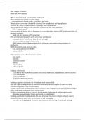
What is a conceptual model?
- Visual representations of relations between theoretical constructs and variables of interest.
- Model: simplified description of reality.
- The boxes represent variables.
- Arrows represent relationships between variables.
- Arrows go from predictor variables to outcome variables.
- Hypotheses refer to specific arrows e.g. relationships/effects/differences.
Levels of measurement of variables
- Categorical: subgroups are indicated by numbers. Made up of categories and names distinct entities.
o Nominal: two or more categories, in no particular order e.g. male and female.
o Ordinal: ordered categories e.g. small, medium, large.
- Quantitative: use numerical scales, with equal distances between values.
o Discrete: can take only certain values e.g. 1, 2, 3.
o Interval: equal intervals on the scale.
o Ratio: true and meaningful zero point e.g. time, income.
- In social sciences, we often treat ordinal scales as interval (pseudo) scales e.g. Likert scales (1 – 5 disagree to agree).
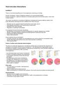
Moderation
- If the proposed effect is stronger in certain settings.
- Also called interaction.
- A moderator is a variable that affects the strength of the relation between
the predictor and outcome variable.
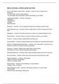
Mediation
- If the proposed relationship goes via another variable.
- A mediating variable explains the relation between the predictor and the
outcome variable.
Hypotheses
- H0: null hypothesis (rejected or not)
- H1: alternative/research hypothesis (supported or not)
- Hypotheses are developed prior to research. They are based on theory and previous research.
- Not all potential relationships need to be hypothesized:
o Every hypothesis refers to an arrow in the conceptual model.
o But not every potential arrow refers to a hypothesis.
- A hypothesis is a verbalized expression of an expected relationship between variables.
1
,One vs. two-sided testing
- If the hypothesis is one-sided, check if the hypothesis is in line with the results (e.g. mean plots).
- If they are in line (e.g. positive and right sided), divide the two tailed p-value by 2.
- If they are not in line, then by (1 – two tailed p-value/2).
Test Hypotheses
- Appropriate way to test hypotheses depends on:
o Nature of the relationship: derived from conceptual model.
• Main effects, moderation/interaction, mediation.
• Total direct, indirect effect.
o Nature of the data: not all of this is derived from conceptual model.
• Number of PV, number of OVs
• How are variables operationalized?
• Data type PVs, data type OVs
• If there are multiple groups: number of groups, relationship between them (dependent/independent).
Independent and Paired Samples T-test
- Paired-samples t tests compare scores on two different variables but for the same group of cases.
- Independent-samples t tests compare scores on the same variable but for two different groups of cases.
o Use when there is one quantitative outcome variable and one categorial predictor variable with two mutually exclusive
categories.
Analysis of Variance – ANOVA
- With ANOVA, we are examining how much of the variance in our data can be explained by our predictor variable.
- ideally 40 observations per group
One-way independent ANOVA
- One-way independent ANOVA: when the participants are different (independent groups) and there is only one predictor
variable.
- Conditions:
o One quantitative outcome variable (when the OV is quantitative – test on the mean)
o One categorical predictor variable
o Two or more mutually exclusive categories/groups (independent groups)
- Assumptions: need to adhere to these assumptions, in order to prevent invalid outcomes.
o Variance is homogeneous across groups.
o Residuals are normally distributed.
o Groups are roughly equal sized.
- Distinguish between:
o Number of categories within one categorial predictor variable.
o Number of predictor variables.
- Hypotheses:
o H0: μ1 = μ2 = … = μi
• i = number of categories
• No difference in OV mean across the different categories in PV.
o H1: at least one μ differs
• There is at least one difference in OV mean score between PV categories.
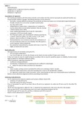
- Based on an F-Test
o Test statistic: F-test
o F-distribution looks different than t-distribution.
o F-values are looking to explain variability.
- ANOVA decomposes total variability observed in OV into variation explained by the model and residual variation.
o Explained variability: how much is caused by differences between groups?
o Unexplained variability: how much is caused by differences within groups?
o Prefer a larger proportion of the variability to be explained than unexplained.
Variability measures
- Variance: the averages of the squared differences from the mean.
- Sum of squares: the sum of the squared differences from the mean.
o Used for ANOVA analysis.
o Use squared deviations because we want positive outcomes.
2
, Sums of squares
SStotal = SSmodel + SSresidual
- Total sum of squares
o Squared deviations from grand overall mean.
o Total variability to be explained.
- Model Sum of Squares
o Between SS: explained variability.
o Squared deviations group means from grand overall mean.
o How much variability can be explained by differences between groups?
- Residual sum of squares
o Unexplained variability: within SS.
o Squared deviations observations from group means.
o How much variation within groups?
o Thus, not explained by the groups we compare.
How to use the sums of squares?
1. R2: proportion of total variance in our data that is “explained” by our model.
!!
o R2 = !!!
"
- Explained variability / total variability
- Model Sum of Squares / Total Sum of Squares
- An important and valuable indication but not a formal statistical test.
2. F-Test
- To investigate if the group means differ with an ANOVA, we do an F-test.
- This is a statistical test and checks the ration explained variability to unexplained variability.
"#$%&'(") +&,'&-'%'./ -".1""( 2,30$ +&,'&-'%'./
o F(ratio) = =
0("#$%&'(") +&,'&-'%'./ 1'.4'( 2,30$ +&,'&-'%'./
- We cannot divide the model sum of square by the residual sum of squares because they are not based on same number of
observations/df.
- We therefore divide by the degrees of freedom to get Mean Squares (MS)
5! !! /)7 !! /89:
o F = 5!! = 5!! /)7! = !! !/((98)
# # # #
- We want a large F value because this means that a larger proportion of the variability is explained.
- Degrees of freedom (df) one-way independent ANOVA:
o dfM = k-1
o dfR = n-k
o dfT = n-1
*k = number of categories
*n = number of observations
From F to p to conclusion H0
- F is a test statistic which means it has both a null hypothesis and an alternative hypothesis.
- From test statistics to p-value:
o From F-ratio to p-value (depends on df)
o Look in F-table for critical value: dfR and dfM
- From (critical) p-value to conclusion H0
o If F-ratio > critical p-value: reject H0
One-way independent ANOVA calculations example
Research question: is there a relation between shopping platform and customer satisfaction?
- PV = shopping platform (categorical) with 3 levels/categories:
o 1 Brick-and-mortar store
o 2 Web shop
o 3 Reseller
- OV = customer satisfaction (quantitative)
o Score from 1-50
- 10 observations – not realistic
- A 1-way independent ANOVA is appropriate because there is one quantitative outcome variable and one categorical
predictor variable with more than two mutually exclusive categories.
H0: μ1 = μ2 = μ3
H1: at least one μ differs
3
LECTURES
WEEK 1
OV = Outcome Variable (Field)
- DV = Dependent Variable: test variable, variable to be explained
PV = Predictor Variable (Field)
- IV = Independent Variable: variable that explains
We are interested of the effect of a predictor variable on an outcome variable.
The p-value
- Stands for the probability of obtaining a result (or test-statistic value) equal to (or ‘more extreme’ than) what was actually
observed (the result you actually got), assuming that the null hypothesis is true.
- P ≤ 0.05
o Reject the null hypothesis and support the alternative hypothesis.
o Given the sample and the significance level of 5% there is sufficient support that the mean weight differs from 12g.
o A low p value indicates that the null hypothesis is unlikely.
- P > 0.05
- Do not reject the null hypothesis and do not support the alternative hypothesis.
- Given the sample and significance level of 5%, there is not sufficient support that the mean weight differs from 12g.
What is a conceptual model?
- Visual representations of relations between theoretical constructs and variables of interest.
- Model: simplified description of reality.
- The boxes represent variables.
- Arrows represent relationships between variables.
- Arrows go from predictor variables to outcome variables.
- Hypotheses refer to specific arrows e.g. relationships/effects/differences.
Levels of measurement of variables
- Categorical: subgroups are indicated by numbers. Made up of categories and names distinct entities.
o Nominal: two or more categories, in no particular order e.g. male and female.
o Ordinal: ordered categories e.g. small, medium, large.
- Quantitative: use numerical scales, with equal distances between values.
o Discrete: can take only certain values e.g. 1, 2, 3.
o Interval: equal intervals on the scale.
o Ratio: true and meaningful zero point e.g. time, income.
- In social sciences, we often treat ordinal scales as interval (pseudo) scales e.g. Likert scales (1 – 5 disagree to agree).
Moderation
- If the proposed effect is stronger in certain settings.
- Also called interaction.
- A moderator is a variable that affects the strength of the relation between
the predictor and outcome variable.
Mediation
- If the proposed relationship goes via another variable.
- A mediating variable explains the relation between the predictor and the
outcome variable.
Hypotheses
- H0: null hypothesis (rejected or not)
- H1: alternative/research hypothesis (supported or not)
- Hypotheses are developed prior to research. They are based on theory and previous research.
- Not all potential relationships need to be hypothesized:
o Every hypothesis refers to an arrow in the conceptual model.
o But not every potential arrow refers to a hypothesis.
- A hypothesis is a verbalized expression of an expected relationship between variables.
1
,One vs. two-sided testing
- If the hypothesis is one-sided, check if the hypothesis is in line with the results (e.g. mean plots).
- If they are in line (e.g. positive and right sided), divide the two tailed p-value by 2.
- If they are not in line, then by (1 – two tailed p-value/2).
Test Hypotheses
- Appropriate way to test hypotheses depends on:
o Nature of the relationship: derived from conceptual model.
• Main effects, moderation/interaction, mediation.
• Total direct, indirect effect.
o Nature of the data: not all of this is derived from conceptual model.
• Number of PV, number of OVs
• How are variables operationalized?
• Data type PVs, data type OVs
• If there are multiple groups: number of groups, relationship between them (dependent/independent).
Independent and Paired Samples T-test
- Paired-samples t tests compare scores on two different variables but for the same group of cases.
- Independent-samples t tests compare scores on the same variable but for two different groups of cases.
o Use when there is one quantitative outcome variable and one categorial predictor variable with two mutually exclusive
categories.
Analysis of Variance – ANOVA
- With ANOVA, we are examining how much of the variance in our data can be explained by our predictor variable.
- ideally 40 observations per group
One-way independent ANOVA
- One-way independent ANOVA: when the participants are different (independent groups) and there is only one predictor
variable.
- Conditions:
o One quantitative outcome variable (when the OV is quantitative – test on the mean)
o One categorical predictor variable
o Two or more mutually exclusive categories/groups (independent groups)
- Assumptions: need to adhere to these assumptions, in order to prevent invalid outcomes.
o Variance is homogeneous across groups.
o Residuals are normally distributed.
o Groups are roughly equal sized.
- Distinguish between:
o Number of categories within one categorial predictor variable.
o Number of predictor variables.
- Hypotheses:
o H0: μ1 = μ2 = … = μi
• i = number of categories
• No difference in OV mean across the different categories in PV.
o H1: at least one μ differs
• There is at least one difference in OV mean score between PV categories.
- Based on an F-Test
o Test statistic: F-test
o F-distribution looks different than t-distribution.
o F-values are looking to explain variability.
- ANOVA decomposes total variability observed in OV into variation explained by the model and residual variation.
o Explained variability: how much is caused by differences between groups?
o Unexplained variability: how much is caused by differences within groups?
o Prefer a larger proportion of the variability to be explained than unexplained.
Variability measures
- Variance: the averages of the squared differences from the mean.
- Sum of squares: the sum of the squared differences from the mean.
o Used for ANOVA analysis.
o Use squared deviations because we want positive outcomes.
2
, Sums of squares
SStotal = SSmodel + SSresidual
- Total sum of squares
o Squared deviations from grand overall mean.
o Total variability to be explained.
- Model Sum of Squares
o Between SS: explained variability.
o Squared deviations group means from grand overall mean.
o How much variability can be explained by differences between groups?
- Residual sum of squares
o Unexplained variability: within SS.
o Squared deviations observations from group means.
o How much variation within groups?
o Thus, not explained by the groups we compare.
How to use the sums of squares?
1. R2: proportion of total variance in our data that is “explained” by our model.
!!
o R2 = !!!
"
- Explained variability / total variability
- Model Sum of Squares / Total Sum of Squares
- An important and valuable indication but not a formal statistical test.
2. F-Test
- To investigate if the group means differ with an ANOVA, we do an F-test.
- This is a statistical test and checks the ration explained variability to unexplained variability.
"#$%&'(") +&,'&-'%'./ -".1""( 2,30$ +&,'&-'%'./
o F(ratio) = =
0("#$%&'(") +&,'&-'%'./ 1'.4'( 2,30$ +&,'&-'%'./
- We cannot divide the model sum of square by the residual sum of squares because they are not based on same number of
observations/df.
- We therefore divide by the degrees of freedom to get Mean Squares (MS)
5! !! /)7 !! /89:
o F = 5!! = 5!! /)7! = !! !/((98)
# # # #
- We want a large F value because this means that a larger proportion of the variability is explained.
- Degrees of freedom (df) one-way independent ANOVA:
o dfM = k-1
o dfR = n-k
o dfT = n-1
*k = number of categories
*n = number of observations
From F to p to conclusion H0
- F is a test statistic which means it has both a null hypothesis and an alternative hypothesis.
- From test statistics to p-value:
o From F-ratio to p-value (depends on df)
o Look in F-table for critical value: dfR and dfM
- From (critical) p-value to conclusion H0
o If F-ratio > critical p-value: reject H0
One-way independent ANOVA calculations example
Research question: is there a relation between shopping platform and customer satisfaction?
- PV = shopping platform (categorical) with 3 levels/categories:
o 1 Brick-and-mortar store
o 2 Web shop
o 3 Reseller
- OV = customer satisfaction (quantitative)
o Score from 1-50
- 10 observations – not realistic
- A 1-way independent ANOVA is appropriate because there is one quantitative outcome variable and one categorical
predictor variable with more than two mutually exclusive categories.
H0: μ1 = μ2 = μ3
H1: at least one μ differs
3