Week 1 Corporate Finance: Nelson Paper Products (Case 1) + Valuation Methods compared
Lecture: Valuation
➔ Valuation is always biased + subjective (based on situation and incentives)
➔ Payoff of valuation is higher with a range/interval rather than a precise value
➔ The easier to interpret (and remodel) a valuation model, the better (simpler models > complex models)
➔ If markets are efficient, economic value = book value
➔ Economic value
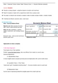
Uses – Sources Balance Sheet
Sources (right side): sources of money =
debt + paid-in equity/retained earnings
Uses (left side): operations + working
capital, investments, cash holdings (excess
cash)
Economic value ~ what (current and future)
benefits assets have
Approaches to value a company
1) Net Asset Approach
Total Assets minus Total Liabilities
Problem: accounting-based values, often very different from market (or current) value
Solutions/Adjustments:
(1) Adjusted Book Value:
re-value tangible assets (compare purchase price and depreciation with current market value)
(2) Liquidation Value: (= Floor Value)
“what would I get if I liquidated everything today?” – this also considers costs of a quick sale
(3) Replacement Value:
Current costs of reproducing/rebuild the tangible assets from scratch right now
,2) Multiples (or Relatives) Approach
Multiple of earnings, EBIT, Sales or book values (industry-average or historic)
EBIT = earning power without effect of financing the company
i. Historical Earnings
ii. Future Earnings under Present Ownerships
iii. Future Earnings under New Ownerships
2 kinds of multiples
(1) Trading Multiples
a. P/E
b. Equity Value/Sales or Equity Value/EBITDA
c. Price/Book = market price per share / book value per share
(2) Transaction Multiples
Higher than trading multiples because it concerns acquisitions of similar companies
Limitations: static measures (every offer/acquisition is different)
Equity vs. Firm Valuation
Discount CF @
equity cost to find
Equity Value
Discount CF @ wacc
to find Enterprise
Value
3) Discounted Dividends Approach
PV of company = perpetuity of cash flows (dividends)
𝐶𝐹𝑝𝑒𝑟 𝑦𝑒𝑎𝑟
𝑃𝑟𝑒𝑠𝑒𝑛𝑡 𝑉𝑎𝑙𝑢𝑒 𝑃𝑉(𝐶𝐹 𝑖𝑛 𝑝𝑒𝑟𝑝𝑒𝑡𝑢𝑖𝑡𝑦 ) =
𝑟
𝐶𝐹1
𝑃𝑟𝑒𝑠𝑒𝑛𝑡 𝑉𝑎𝑙𝑢𝑒 𝑃𝑉(𝑔𝑟𝑜𝑤𝑖𝑛𝑔 𝑝𝑒𝑟𝑝𝑒𝑡𝑢𝑖𝑡𝑦) =
𝑟−𝑔
, 𝐶 1
𝑃𝑟𝑒𝑠𝑒𝑛𝑡 𝑉𝑎𝑙𝑢𝑒 𝑃𝑉(𝑁 𝑝𝑒𝑟𝑖𝑜𝑑𝑠) = (1 − )
𝑟 (1 + 𝑟)𝑁
𝐶 1+𝑔 𝑁
𝑃𝑟𝑒𝑠𝑒𝑛𝑡 𝑉𝑎𝑙𝑢𝑒 𝑃𝑉(𝐶 𝑔𝑟𝑜𝑤𝑖𝑛𝑔 𝑏𝑦 𝑔 𝑓𝑜𝑟 𝑁 𝑝𝑒𝑟𝑖𝑜𝑑𝑠) = (1 − ( ) )
𝑟−𝑔 1+𝑟
𝑁
𝐷𝑖𝑣 1 + 𝑔1 1 𝐷𝑖𝑣 𝑁 (1 + 𝑔2
𝑃𝑉(𝑔𝑟𝑜𝑤𝑖𝑛𝑔𝑎𝑛𝑛𝑢𝑖𝑡𝑦 + 𝑝𝑒𝑟𝑝𝑒𝑡𝑢𝑖𝑡𝑦𝑎𝑓𝑡𝑒𝑟𝑦𝑒𝑎𝑟𝑁) = (1 − ( ) ) + ∗ ( )
𝑟 − 𝑔1 1+𝑟 (1 + 𝑟)𝑁 𝑟 − 𝑔2
𝐷𝑖𝑣 𝑁 (1 + 𝑔2
𝑤ℎ𝑒𝑟𝑒 ( ) = 𝑇𝑒𝑟𝑚𝑖𝑛𝑎𝑙 𝑉𝑎𝑙𝑢𝑒
𝑟 − 𝑔2
𝐷𝑖𝑣1 1 + 𝑔1 𝑛 1 + 𝑔2 𝑛 (𝐷𝑖𝑣1 )
= 𝑃0 = ∗ (1 − ( ) )+( ) ∗
𝑟 − 𝑔1 1+𝑟 1+𝑟 (𝑟 − 𝑔2 )
Terminal Value after period n
Limitations:
1. If g > r (wacc) then discount model does not work
2. does not work with unstable payout pattern
Cash Flow Valuation Methods
Valuation always dependent on 2 main elements:
(1) Assessment of (incremental) future cash flow
(2) discount rate that reflects the risk involved
𝐶𝐹
𝑡
Basic: 𝑃𝑉 = ∑ (1+𝑟) 𝑡
𝐶𝐹𝑝𝑒𝑟 𝑦𝑒𝑎𝑟
Perpetuity: 𝑃𝑉(𝐶𝐹 𝑖𝑛 𝑝𝑒𝑟𝑝𝑒𝑡𝑢𝑖𝑡𝑦 ) = 𝑟
𝐶𝐹
Constant Growth Perpetuity: 𝑃𝑉(𝑔𝑟𝑜𝑤𝑖𝑛𝑔 𝑝𝑒𝑟𝑝𝑒𝑡𝑢𝑖𝑡𝑦 ) = 𝑟−𝑔1
Changing growth rates (estimating cash flows for the first years and then constant (lower) growth perpetuity)
𝐶𝐹𝑡 𝐶𝐹𝑡
𝑃𝑉 = ∑ 𝑡
+ ( ) / (1 + 𝑟)𝑡
(1 + 𝑟) 𝑟 − 𝑔
,Growing Annuity and then growing perpetuity
𝐷𝑖𝑣 𝑁 (1 + 𝑔2
𝐷𝑖𝑣 1+𝑔 1 𝑁 ( )
𝑟 − 𝑔2
(1 − ( ) )+
𝑟 − 𝑔1 1+𝑟 (1 + 𝑟)𝑁
EXCEL =PV(rate, periods, payment,0,0)
(1) Free Cash Flow FCF
FCF = EBIT (1 – tax rate) + Depreciation – Capital Expenditure - ∆Working Capital
- Unlevered cash flow as debt payments are not considered
(2) Discount Rate (required return ~ opportunity cost)
According to CAPM – expect rate of return on equity 𝑟𝑒 = 𝑟𝑓 + 𝛽𝑓 ( 𝐸(𝑟𝑚 ) − 𝑟𝑓 )
(WACC) Weighted Average Cost of Capital
𝑈𝑛𝑙𝑒𝑣𝑒𝑟𝑒𝑑 𝐶𝐹𝑝𝑒𝑟 𝑦𝑒𝑎𝑟
𝑁𝑃𝑉 = − 𝑖𝑛𝑖𝑡𝑖𝑎𝑙 𝑖𝑛𝑣𝑒𝑠𝑡𝑚𝑒𝑛𝑡
𝑟𝑤𝑎𝑐𝑐
But expected rate of return on equity also depends on financial leverage of firm
The more leverage, the higher the expected return on the equity
𝑬 𝑫 𝑫
After-tax WACC: 𝒓𝒘𝒂𝒄𝒄 = 𝑬+𝑫 𝒓𝑬 + 𝑬+𝑫 𝒓𝑫 (𝟏 − 𝝉𝒄 ) = 𝒓𝑼 − 𝑽 ∗ 𝝉𝒄 ∗ 𝒓𝑫
𝑫
(𝑎𝑓𝑡𝑒𝑟 𝑡𝑎𝑥 𝑤𝑖𝑡ℎ 𝑙𝑒𝑣𝑒𝑟𝑎𝑔𝑒) 𝒓𝒆 = 𝒓𝒖 + (𝟏 − 𝒕𝒄 )(𝒓𝒖 − 𝒓𝒅 )
𝑬
𝑫
(𝑝𝑟𝑒 − 𝑡𝑎𝑥 𝑤𝑖𝑡ℎ 𝑙𝑒𝑣𝑒𝑟𝑎𝑔𝑒) 𝑟𝑒 = 𝒓𝒖 + (𝒓 − 𝒓𝒅 )
𝑬 𝒖
𝑟𝑑 = 𝑖𝑛𝑡𝑒𝑟𝑒𝑠𝑡 𝑟𝑎𝑡𝑒 𝑜𝑛 𝑑𝑒𝑏𝑡 𝑐𝑎𝑝𝑖𝑡𝑎𝑙
➔ Values for debt and Equity in WACC model
are market values not, book values
➔ WACC most useful when tax and debt
structure do not change over time
, Cost of Capital of Levered Equity Same for beta:
𝐷
𝛽𝐸 = 𝛽𝑈 + ( ) ∗ (𝛽𝑈 − 𝛽𝐷 )
𝐸
𝐷
𝑟𝐸 = 𝑟𝑈 + ( ) ∗ (𝑟𝑈 − 𝑟𝐷 )
𝐸
𝐸
𝛽𝐴 = 𝛽𝐸 ∗ (𝑉) if debt = risk-free
4) Discounted Cash Flow
1. Discounted Cash Flow
Valuation always dependent on 2 main elements:
(1) Assessment of (incremental) future cash flow
(2) discount rate that reflects the risk involved (opportunity cost)
➔ Enterprise Value = Market Value of Equity + Debt – Cash
(Enterprise Value = Assets that are not (liquid) cash)
➔ Free Cash Flow Valuation
𝐹𝑟𝑒𝑒 𝐶𝑎𝑠ℎ 𝐹𝑙𝑜𝑤 = 𝐸𝐵𝐼𝑇 (1 − 𝜏𝑐 ) + 𝐷𝑒𝑝𝑟𝑒𝑐𝑖𝑎𝑡𝑖𝑜𝑛 − 𝐶𝑎𝑝𝐸𝑥. − ∆𝑁𝑊𝐶
𝐸𝑛𝑡𝑒𝑟𝑝𝑟𝑖𝑠𝑒 𝑉𝑎𝑙𝑢𝑒 + 𝐶𝑎𝑠ℎ − 𝐷𝑒𝑏𝑡
𝑃𝑟𝑖𝑐𝑒 𝑜𝑓 𝑆ℎ𝑎𝑟𝑒 =
𝑆ℎ𝑎𝑟𝑒𝑠 𝑂𝑢𝑡𝑠𝑡𝑎𝑛𝑑𝑖𝑛𝑔
➔ Continuation/Terminal Value
𝐹𝐶𝐹1 𝐹𝐶𝐹𝑛 + 𝑉𝑛 1 + 𝑔𝐹𝐶𝐹
𝑉0 = +⋯+ 𝑉𝑛 = 𝐹𝐶𝐹𝑛 ∗ ( )
1 + 𝑟𝑤𝑎𝑐𝑐 (1 + 𝑟𝑤𝑎𝑐𝑐 )𝑛 𝑟𝑤𝑎𝑐𝑐 − 𝑔𝐹𝐶𝐹
Limitations:
1. Need for positive FCF to evaluate its value
2. Early cash flows producing assets are worth more than equivalent assets with FCF later
Capital Cash Flow (enterprise value)
4 steps
a) Construct future cash flows
b) Calculate terminal value
c) Determine appropriate discount rate
d) Getting the equity value (~Enterprise value – Debt)
(CCF) Capital Cash Flow
E D
= Pre-tax WACC rU = (E+D) ∗ rE + (E+D) ∗ rD
Lecture: Valuation
➔ Valuation is always biased + subjective (based on situation and incentives)
➔ Payoff of valuation is higher with a range/interval rather than a precise value
➔ The easier to interpret (and remodel) a valuation model, the better (simpler models > complex models)
➔ If markets are efficient, economic value = book value
➔ Economic value
Uses – Sources Balance Sheet
Sources (right side): sources of money =
debt + paid-in equity/retained earnings
Uses (left side): operations + working
capital, investments, cash holdings (excess
cash)
Economic value ~ what (current and future)
benefits assets have
Approaches to value a company
1) Net Asset Approach
Total Assets minus Total Liabilities
Problem: accounting-based values, often very different from market (or current) value
Solutions/Adjustments:
(1) Adjusted Book Value:
re-value tangible assets (compare purchase price and depreciation with current market value)
(2) Liquidation Value: (= Floor Value)
“what would I get if I liquidated everything today?” – this also considers costs of a quick sale
(3) Replacement Value:
Current costs of reproducing/rebuild the tangible assets from scratch right now
,2) Multiples (or Relatives) Approach
Multiple of earnings, EBIT, Sales or book values (industry-average or historic)
EBIT = earning power without effect of financing the company
i. Historical Earnings
ii. Future Earnings under Present Ownerships
iii. Future Earnings under New Ownerships
2 kinds of multiples
(1) Trading Multiples
a. P/E
b. Equity Value/Sales or Equity Value/EBITDA
c. Price/Book = market price per share / book value per share
(2) Transaction Multiples
Higher than trading multiples because it concerns acquisitions of similar companies
Limitations: static measures (every offer/acquisition is different)
Equity vs. Firm Valuation
Discount CF @
equity cost to find
Equity Value
Discount CF @ wacc
to find Enterprise
Value
3) Discounted Dividends Approach
PV of company = perpetuity of cash flows (dividends)
𝐶𝐹𝑝𝑒𝑟 𝑦𝑒𝑎𝑟
𝑃𝑟𝑒𝑠𝑒𝑛𝑡 𝑉𝑎𝑙𝑢𝑒 𝑃𝑉(𝐶𝐹 𝑖𝑛 𝑝𝑒𝑟𝑝𝑒𝑡𝑢𝑖𝑡𝑦 ) =
𝑟
𝐶𝐹1
𝑃𝑟𝑒𝑠𝑒𝑛𝑡 𝑉𝑎𝑙𝑢𝑒 𝑃𝑉(𝑔𝑟𝑜𝑤𝑖𝑛𝑔 𝑝𝑒𝑟𝑝𝑒𝑡𝑢𝑖𝑡𝑦) =
𝑟−𝑔
, 𝐶 1
𝑃𝑟𝑒𝑠𝑒𝑛𝑡 𝑉𝑎𝑙𝑢𝑒 𝑃𝑉(𝑁 𝑝𝑒𝑟𝑖𝑜𝑑𝑠) = (1 − )
𝑟 (1 + 𝑟)𝑁
𝐶 1+𝑔 𝑁
𝑃𝑟𝑒𝑠𝑒𝑛𝑡 𝑉𝑎𝑙𝑢𝑒 𝑃𝑉(𝐶 𝑔𝑟𝑜𝑤𝑖𝑛𝑔 𝑏𝑦 𝑔 𝑓𝑜𝑟 𝑁 𝑝𝑒𝑟𝑖𝑜𝑑𝑠) = (1 − ( ) )
𝑟−𝑔 1+𝑟
𝑁
𝐷𝑖𝑣 1 + 𝑔1 1 𝐷𝑖𝑣 𝑁 (1 + 𝑔2
𝑃𝑉(𝑔𝑟𝑜𝑤𝑖𝑛𝑔𝑎𝑛𝑛𝑢𝑖𝑡𝑦 + 𝑝𝑒𝑟𝑝𝑒𝑡𝑢𝑖𝑡𝑦𝑎𝑓𝑡𝑒𝑟𝑦𝑒𝑎𝑟𝑁) = (1 − ( ) ) + ∗ ( )
𝑟 − 𝑔1 1+𝑟 (1 + 𝑟)𝑁 𝑟 − 𝑔2
𝐷𝑖𝑣 𝑁 (1 + 𝑔2
𝑤ℎ𝑒𝑟𝑒 ( ) = 𝑇𝑒𝑟𝑚𝑖𝑛𝑎𝑙 𝑉𝑎𝑙𝑢𝑒
𝑟 − 𝑔2
𝐷𝑖𝑣1 1 + 𝑔1 𝑛 1 + 𝑔2 𝑛 (𝐷𝑖𝑣1 )
= 𝑃0 = ∗ (1 − ( ) )+( ) ∗
𝑟 − 𝑔1 1+𝑟 1+𝑟 (𝑟 − 𝑔2 )
Terminal Value after period n
Limitations:
1. If g > r (wacc) then discount model does not work
2. does not work with unstable payout pattern
Cash Flow Valuation Methods
Valuation always dependent on 2 main elements:
(1) Assessment of (incremental) future cash flow
(2) discount rate that reflects the risk involved
𝐶𝐹
𝑡
Basic: 𝑃𝑉 = ∑ (1+𝑟) 𝑡
𝐶𝐹𝑝𝑒𝑟 𝑦𝑒𝑎𝑟
Perpetuity: 𝑃𝑉(𝐶𝐹 𝑖𝑛 𝑝𝑒𝑟𝑝𝑒𝑡𝑢𝑖𝑡𝑦 ) = 𝑟
𝐶𝐹
Constant Growth Perpetuity: 𝑃𝑉(𝑔𝑟𝑜𝑤𝑖𝑛𝑔 𝑝𝑒𝑟𝑝𝑒𝑡𝑢𝑖𝑡𝑦 ) = 𝑟−𝑔1
Changing growth rates (estimating cash flows for the first years and then constant (lower) growth perpetuity)
𝐶𝐹𝑡 𝐶𝐹𝑡
𝑃𝑉 = ∑ 𝑡
+ ( ) / (1 + 𝑟)𝑡
(1 + 𝑟) 𝑟 − 𝑔
,Growing Annuity and then growing perpetuity
𝐷𝑖𝑣 𝑁 (1 + 𝑔2
𝐷𝑖𝑣 1+𝑔 1 𝑁 ( )
𝑟 − 𝑔2
(1 − ( ) )+
𝑟 − 𝑔1 1+𝑟 (1 + 𝑟)𝑁
EXCEL =PV(rate, periods, payment,0,0)
(1) Free Cash Flow FCF
FCF = EBIT (1 – tax rate) + Depreciation – Capital Expenditure - ∆Working Capital
- Unlevered cash flow as debt payments are not considered
(2) Discount Rate (required return ~ opportunity cost)
According to CAPM – expect rate of return on equity 𝑟𝑒 = 𝑟𝑓 + 𝛽𝑓 ( 𝐸(𝑟𝑚 ) − 𝑟𝑓 )
(WACC) Weighted Average Cost of Capital
𝑈𝑛𝑙𝑒𝑣𝑒𝑟𝑒𝑑 𝐶𝐹𝑝𝑒𝑟 𝑦𝑒𝑎𝑟
𝑁𝑃𝑉 = − 𝑖𝑛𝑖𝑡𝑖𝑎𝑙 𝑖𝑛𝑣𝑒𝑠𝑡𝑚𝑒𝑛𝑡
𝑟𝑤𝑎𝑐𝑐
But expected rate of return on equity also depends on financial leverage of firm
The more leverage, the higher the expected return on the equity
𝑬 𝑫 𝑫
After-tax WACC: 𝒓𝒘𝒂𝒄𝒄 = 𝑬+𝑫 𝒓𝑬 + 𝑬+𝑫 𝒓𝑫 (𝟏 − 𝝉𝒄 ) = 𝒓𝑼 − 𝑽 ∗ 𝝉𝒄 ∗ 𝒓𝑫
𝑫
(𝑎𝑓𝑡𝑒𝑟 𝑡𝑎𝑥 𝑤𝑖𝑡ℎ 𝑙𝑒𝑣𝑒𝑟𝑎𝑔𝑒) 𝒓𝒆 = 𝒓𝒖 + (𝟏 − 𝒕𝒄 )(𝒓𝒖 − 𝒓𝒅 )
𝑬
𝑫
(𝑝𝑟𝑒 − 𝑡𝑎𝑥 𝑤𝑖𝑡ℎ 𝑙𝑒𝑣𝑒𝑟𝑎𝑔𝑒) 𝑟𝑒 = 𝒓𝒖 + (𝒓 − 𝒓𝒅 )
𝑬 𝒖
𝑟𝑑 = 𝑖𝑛𝑡𝑒𝑟𝑒𝑠𝑡 𝑟𝑎𝑡𝑒 𝑜𝑛 𝑑𝑒𝑏𝑡 𝑐𝑎𝑝𝑖𝑡𝑎𝑙
➔ Values for debt and Equity in WACC model
are market values not, book values
➔ WACC most useful when tax and debt
structure do not change over time
, Cost of Capital of Levered Equity Same for beta:
𝐷
𝛽𝐸 = 𝛽𝑈 + ( ) ∗ (𝛽𝑈 − 𝛽𝐷 )
𝐸
𝐷
𝑟𝐸 = 𝑟𝑈 + ( ) ∗ (𝑟𝑈 − 𝑟𝐷 )
𝐸
𝐸
𝛽𝐴 = 𝛽𝐸 ∗ (𝑉) if debt = risk-free
4) Discounted Cash Flow
1. Discounted Cash Flow
Valuation always dependent on 2 main elements:
(1) Assessment of (incremental) future cash flow
(2) discount rate that reflects the risk involved (opportunity cost)
➔ Enterprise Value = Market Value of Equity + Debt – Cash
(Enterprise Value = Assets that are not (liquid) cash)
➔ Free Cash Flow Valuation
𝐹𝑟𝑒𝑒 𝐶𝑎𝑠ℎ 𝐹𝑙𝑜𝑤 = 𝐸𝐵𝐼𝑇 (1 − 𝜏𝑐 ) + 𝐷𝑒𝑝𝑟𝑒𝑐𝑖𝑎𝑡𝑖𝑜𝑛 − 𝐶𝑎𝑝𝐸𝑥. − ∆𝑁𝑊𝐶
𝐸𝑛𝑡𝑒𝑟𝑝𝑟𝑖𝑠𝑒 𝑉𝑎𝑙𝑢𝑒 + 𝐶𝑎𝑠ℎ − 𝐷𝑒𝑏𝑡
𝑃𝑟𝑖𝑐𝑒 𝑜𝑓 𝑆ℎ𝑎𝑟𝑒 =
𝑆ℎ𝑎𝑟𝑒𝑠 𝑂𝑢𝑡𝑠𝑡𝑎𝑛𝑑𝑖𝑛𝑔
➔ Continuation/Terminal Value
𝐹𝐶𝐹1 𝐹𝐶𝐹𝑛 + 𝑉𝑛 1 + 𝑔𝐹𝐶𝐹
𝑉0 = +⋯+ 𝑉𝑛 = 𝐹𝐶𝐹𝑛 ∗ ( )
1 + 𝑟𝑤𝑎𝑐𝑐 (1 + 𝑟𝑤𝑎𝑐𝑐 )𝑛 𝑟𝑤𝑎𝑐𝑐 − 𝑔𝐹𝐶𝐹
Limitations:
1. Need for positive FCF to evaluate its value
2. Early cash flows producing assets are worth more than equivalent assets with FCF later
Capital Cash Flow (enterprise value)
4 steps
a) Construct future cash flows
b) Calculate terminal value
c) Determine appropriate discount rate
d) Getting the equity value (~Enterprise value – Debt)
(CCF) Capital Cash Flow
E D
= Pre-tax WACC rU = (E+D) ∗ rE + (E+D) ∗ rD