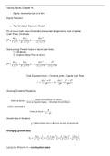
- Equity: ownership right of a firm
Equity Valuation
• The Dividend Discount Model
PV of future cash flows (Dividends) discounted at opportunity cost of capital
Cash Flows: Dividends
𝐷𝑖𝑣₁ 𝐷𝑖𝑣₂ 𝐷𝑖𝑣 𝑛
𝑃0 = + + ⋯ +
1 + 𝑟 𝑒 (1 + 𝑟 𝑒 )2 (1 + 𝑟 𝑒 )𝑛
Stock pricing Present Value of future cash flows
1) Dividends
2) (higher) Sales Price at time n
0
𝐷𝑖𝑣₁ 𝐷𝑖𝑣₂ 𝐷𝑖𝑣 𝑛 𝑃𝑛
𝑃 = + + ⋯+ +
1 + 𝑟 𝑒 (1 + 𝑟 𝑒 )2 (1 + 𝑟 𝑒 )𝑛 (1 + 𝑟 𝑒 )𝑛
Total Expected return = Dividend yield + Capital Gain Rate
𝐷𝑖𝑣1 + 𝑃1 𝐷𝑖𝑣1 𝑃1 − 𝑃0
𝑟= −1 = 0 +
𝑃0 𝑃 𝑃0
Growing Dividend (Perpetuity)
Growth rate of Dividend
𝑔 = 𝑅𝑒𝑡𝑒𝑛𝑡𝑖𝑜𝑛 𝑟𝑎𝑡𝑒 𝑥 𝑅𝑒𝑡𝑢𝑟𝑛 𝑜𝑛 𝑛𝑒𝑤 𝐼𝑛𝑣𝑒𝑠𝑡𝑚𝑒𝑛𝑡
Changing growth rates
𝐷𝑖𝑣1 1 + 𝑔1 𝑛 1 + 𝑔1 𝑛 (𝐷𝑖𝑣1 )
𝑃0 = ∗ (1 − ( ) )+( ) ∗
𝑟 − 𝑔1 1+𝑟 1+𝑟 (𝑟 − 𝑔2 )
Last price (Price N+1) = continuation value
,Payout Ratio = Dividends/Earnings
𝐸𝑎𝑟𝑛𝑖𝑛𝑔
𝐷𝑖𝑣𝑖𝑑𝑒𝑛𝑑 𝑝𝑒𝑟 𝑠ℎ𝑎𝑟𝑒 = 𝑥 𝐷𝑖𝑣𝑖𝑑𝑒𝑛𝑑 𝑃𝑎𝑦𝑜𝑢𝑡 𝑟𝑎𝑡𝑒
𝑠ℎ𝑎𝑟𝑒𝑠 𝑂𝑢𝑡𝑠𝑡𝑎𝑛𝑑𝑖𝑛𝑔
3 ways to increase dividends
1) Increase earnings
2) Increase dividend payout rate
3) Buy back shares (decrease shares outstanding)
1) Retained Earnings (reinvest in company)
Plowback Ratio, retention Rate
• Total Payout and free Cash Flow Valuation
𝑃𝑉 (𝐹𝑢𝑡𝑢𝑟𝑒 𝑇𝑜𝑡𝑎𝑙 𝐷𝑖𝑣𝑖𝑑𝑒𝑛𝑑𝑠 𝑎𝑛𝑑 𝑅𝑒𝑝𝑢𝑟𝑐ℎ𝑎𝑠𝑒𝑠)
𝑇𝑜𝑡𝑎𝑙 𝑃𝑎𝑦𝑜𝑢𝑡 𝑀𝑜𝑑𝑒𝑙 =
𝑆ℎ𝑎𝑟𝑒𝑠 𝑂𝑢𝑡𝑠𝑡𝑎𝑛𝑑𝑖𝑛𝑔
(if firm pays out all of its net profit as dividends)
Discounted Free Cash Flow Model
➔ Enterprise Value = Market Value of Equity + Debt – Cash
(Enterprise Value = Assets that are not (liquid) cash)
➔ Free Cash Flow Valuation
𝐹𝑟𝑒𝑒 𝐶𝑎𝑠ℎ 𝐹𝑙𝑜𝑤 = 𝐸𝐵𝐼𝑇 (1 − 𝜏𝑐 ) + 𝐷𝑒𝑝𝑟𝑒𝑐𝑖𝑎𝑡𝑖𝑜𝑛 − 𝐶𝑎𝑝𝐸𝑥. − ∆𝑁𝑊𝐶
𝐸𝑛𝑡𝑒𝑟𝑝𝑟𝑖𝑠𝑒 𝑉𝑎𝑙𝑢𝑒 + 𝐶𝑎𝑠ℎ − 𝐷𝑒𝑏𝑡
𝑃𝑟𝑖𝑐𝑒 𝑜𝑓 𝑆ℎ𝑎𝑟𝑒 =
𝑆ℎ𝑎𝑟𝑒𝑠 𝑂𝑢𝑡𝑠𝑡𝑎𝑛𝑑𝑖𝑛𝑔
➔ Continuation Value
𝐹𝐶𝐹1 𝐹𝐶𝐹𝑛 + 𝑉𝑛
𝑉0 = +⋯+
1 + 𝑟𝑤𝑎𝑐𝑐 (1 + 𝑟𝑤𝑎𝑐𝑐 )𝑛
𝐹𝐶𝐹𝑛
𝑉𝑛 = ( )
𝑟𝑤𝑎𝑐𝑐 − 𝑔𝐹𝐶𝐹
, • Valuation based on comparable Firms
Using multiples like P/E or P/B or Enterprise Value/Revenue
Does not consider important differences among firms in the same industry
𝑀𝑎𝑟𝑘𝑒𝑡 𝐶𝑎𝑝 𝑆ℎ𝑎𝑟𝑒 𝑃𝑟𝑖𝑐𝑒
𝑃𝑟𝑖𝑐𝑒 𝑡𝑜 𝐸𝑎𝑟𝑛𝑖𝑛𝑔𝑠 𝑅𝑎𝑡𝑖𝑜 𝑃/𝐸 = =
𝑁𝑒𝑡 𝐼𝑛𝑐𝑜𝑚𝑒 𝐸𝑎𝑟𝑛𝑖𝑛𝑔𝑠 𝑝𝑒𝑟 𝑆ℎ𝑎𝑟𝑒
𝑃 𝑃0 𝐷𝑖𝑣𝑖𝑑𝑒𝑛𝑑 𝑃𝑎𝑦𝑜𝑢𝑡 𝑅𝑎𝑡𝑒
𝐹𝑜𝑟𝑤𝑎𝑟𝑑 = 1
=
𝐸 𝐸𝑃𝑆 𝑟−𝑔
Forward P/E Ratio based on expected Earnings in the next 12 months
Most useful comparable = EV/Sales
Efficient market Hypothesis
= relevant information is quickly (almost instantly) and correctly incorporated into the prices of
securities
Securities are priced based on their future cash flows
Securities with equivalent risk have the same expected return
Implications for Corporate Managers:
1) Focus on NPV and Free Cash Flow
2) Focus on free cash flows and not accounting earnings
With efficient markets, accounting decisions don’t always affect value of the firm
3) Use financial transactions to fund investment (liquidity provided by financial markets)
,Chapter 12: Estimating the cost of Capital
Equity cost of capital rule of thumb → 𝑟𝐸 = 𝐷𝑖𝑣. 𝑌𝑖𝑒𝑙𝑑 + 𝐶𝑎𝑝𝑖𝑡𝑎𝑙 𝐺𝑎𝑖𝑛
CAPM (Equity Cost of Capital for an investment)
𝑟 𝑖 = 𝑟 𝑟𝑖𝑠𝑘 𝑓𝑟𝑒𝑒 + 𝛽 (𝐸[𝑅𝑚𝑎𝑟𝑘𝑒𝑡 ] − 𝑟 𝑟𝑖𝑠𝑘 𝑓𝑟𝑒𝑒 )
Components needed for this equation:
1) Market portfolio and its Excess Return over risk free interest rate (= market premium)
2) The investment’s beta (= sensitivity to the market portfolio)
1. Market Portfolio = Index (= Market Proxy)
Weighted values of companies in the Index
(Market Cap Firm i) / (Total Market Caps in the Index)
Indices like S&P 500, Nasdaq, Dow Jones, DAX 30, FTSE 100
2. Risk Free Return Rate
US Treasury Securities
3. Beta
best fitting regression line in between a security’s excess return and the market’s
excess return
Linear regression
(𝑅𝑖 − 𝑟 𝑟𝑖𝑠𝑘 𝑓𝑟𝑒𝑒 ) = 𝛼 𝑖 + 𝛽 𝑖 (𝑅𝑀𝑎𝑟𝑘𝑒𝑡 − 𝑟 𝑟𝑖𝑠𝑘 𝑓𝑟𝑒𝑒 ) + 𝑒 𝑖
Excess Return Company i = Intercept of regression line + sensitivity of i + deviation from the line
, 𝐸[𝑅𝑖 ] = 𝑟 𝑟𝑖𝑠𝑘 𝑓𝑟𝑒𝑒 + 𝛽 (𝐸[𝑅𝑚𝑎𝑟𝑘𝑒𝑡 ] − 𝑟 𝑟𝑖𝑠𝑘 𝑓𝑟𝑒𝑒 ) + 𝛼 𝑖
Expected Return i = Expected return for i from SML + Distance above/below the SML
Improving a portfolio by buying stocks with a positive alpha α and selling those with a negative
alpha α
𝐴𝑙𝑝ℎ𝑎 𝑜𝑓 𝑎 𝑠𝑡𝑜𝑐𝑘 𝛼 = 𝐸 [𝑅] − 𝑟𝑒𝑞𝑢𝑖𝑟𝑒𝑑 𝑅
Alpha of a stock = its deviation (distance) from the security market line
Security market line = capital market line = efficient (market) portfolio frontier
Asset (or Unlevered) beta
𝐸 𝐷
𝛽𝑈 = 𝛽 𝐴 = ∗ 𝛽𝐸 + ∗ 𝛽𝐷
𝐸+𝐷 𝐸+𝐷
The Debt Cost of Capital
𝑟𝑒𝑞𝑢𝑖𝑟𝑒𝑑 𝑟𝑒𝑡𝑢𝑟𝑛 𝑜𝑛 𝑏𝑜𝑛𝑑 𝑟 𝑑 = 𝑌𝑖𝑒𝑙𝑑 𝑡𝑜 𝑀𝑎𝑡𝑢𝑟𝑖𝑡𝑦 − 𝑃𝑟𝑜𝑏𝑎𝑏𝑖𝑙𝑖𝑡𝑦(𝑑𝑒𝑓𝑎𝑢𝑙𝑡 ) ∗ 𝐸𝑥𝑝𝑒𝑐𝑡𝑒𝑑 𝐿𝑜𝑠𝑠 𝑅𝑎𝑡𝑒
Weighted Average Cost of Capital (after-tax) WACC
𝐸 𝐷 𝐷
r wacc = 𝑟𝐸 + 𝑟 𝐷 (1 − 𝜏 𝑐 ) = 𝑟𝑈 − ∗ 𝜏𝑐 ∗ 𝑟𝐷
𝐸+𝐷 𝐸+𝐷 𝐸


