Lecture 1 (02-02-2021) – Value Drivers
The economic value of the firm is the discounted sum of expected future cash flows. Economic value,
however, is not necessarily equal to market value.
The three steps of equity valuation:
1. Understanding the past
2. Forecasting the future
3. Valuation
What is the maximum you are willing to pay for an investment that you expect to yield EUR 100 for
three years while a comparable risky investment is expected to return 8% per year? Answer:
CF 1 CF 2 CF 3 100 100 100
V 0=Ε 0
[ ( 1+r ) 1
+
(1+r ) 2
+
( 1+ r ) 3
] [
=Ε + +
]
( 1+ 0.08 ) ( 1+0.08 ) ( 1+0.08 )3
1 2
=257.71.
The value of an equity interest is based on the present value of the expected future cash dividends to be
∞
DI V t
received: P0=E 0
[ ( )]
∑
t=1 ( 1+r )t
, where P0 is the value of the common equity at time 0, DIVt is the
amount of cash dividends to be paid in period t, r is the discount rate, and E0 [·] indicates that what’s
inside the brackets is uncertain (i.e., expected values). The dividend discount formula is rarely used
directly, because (1) dividends do not directly reflect performance (a firm can also pay out dividends
when it is making a loss), (2) dividends are to a large extent discretionary, and (3) many firms do not pay
dividend right now but promise to pay later.
Periodic return and re-investment:
, ∞
DI V t
Recall that P0=E 0
[ ( )]
∑
t=1 ( 1+r )t
. Generally, C E t =C E t−1 + N I t −DI V t (where CE is the book value of
common equity and NI is net income), so DI V t =N I t −ΔC E t . Plugging this into the first formula and
∞ ∞
N I t −r ∙C Et−1 ( Ro E t−r ) ∙ C E t−1
simplifying yields P0=C E0 + E0
[ ∑
t =1 ( 1+r )
t
]
=C E 0 + E0
[ ∑
t=1 ( 1+r )
t
] , where RoE
is the return on equity (NI / CE).
∞
( Ro E t −r ) ∙C E t−1
Direct inputs to P0=C E0 + E0
[ ∑
t =1 ( 1+r )
t
] are the core value drivers. We distinguish
investment growth (g), risk (r), and profitability (RoE).
Profitability
o Return on equity (RoE) is the key profitability measure. It is the Return on Investment
Earnings for the period
(RoI) for equity investors. RoI = .
Investment at thebeginning of the period
o RoE is the rate of return that equity owners get. RoE must be higher than the
opportunity cost (r) in order to generate value; only if RoE is greater than r, the firm
creates value. We call this opportunity cost (r) ‘expected return’ or ‘cost of equity
capital’.
o When looking at the RoE over time, we see that the mean RoE generally increased as of
1968, but then decreased again from about 1990 onwards. Next to that, its spread has
increased considerably over time. Business and accounting changes affected RoE.
Investment growth
o Besides profitability, the amount of capital invested is also crucial. Investment
depreciates and becomes obsolete: investments need to grow to expand the business,
and investments in new assets are needed to not become obsolete and to stay
competitive.
Risk
o It is quite difficult to forecast next year’s payoff because of a high degree of volatility.
Equity investing, relative to long-term Treasury bills, is therefore quite risky.
o Expected values are uncertain. To adjust for the uncertainty (riskiness) of expectations,
we discount them: r is our measure of this uncertainty. However, coming up with the
right (‘true’) discount rate, r, is challenging. You could use asset pricing models for this.
If we assume that profitability is constant, Ro Et +1=Ro E t =RoE , and capital grows by g each year,
C E t=( 1+ g ) C Et −1, then our basic earnings-based valuation formula simplifies a lot:
∞
( Ro E t −r ) ∙C E t−1 ( Ro E1−r ) ∙C E 0 ( Ro E 1−r ) ∙ ( 1+ g ) C E 0 ( Ro
P0=C E0 + E0
[ ∑
t =1 ( 1+r )
t
]=C E 0+ E0
[ ( 1+r )
1
+
( 1+r )
2
]
+ … =C E0 + E0 [
. You could also rewrite this formula such that the implied growth rate becomes the unknown variable
on the left-hand side of the formula. Then for several discount rates, you can tabulate the corresponding
growth rates.
,Lecture 2 (05-02-2021) – Practice Session
∞
( Ro E t −r ) ∙C E t−1
Direct inputs to P0=C E0 + E0
[ ∑
t =1 ( 1+r )
t
] are the core value drives. We have three value
drivers: growth (g), profitability (RoE), and risk (r). A profitability of 10% does not say that much. You
have to compare it with company’s cost of capital (which reflects the company’s riskiness); if that one is
also 10%, the company does not generate any value. But if it is 5%, the company generates value. If the
investment growth (g) changes, the cost of capital (r) is likely to change as well.
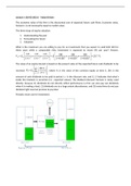
Earnings announcements are the single most important information event, both in terms of absolute
returns as well as share turnover. Those announcements in the third quarter are the most important
ones, because most firms first provide details on next year in the third quarter.
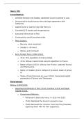
On September 21, 2000, Intel released an
earnings warning. On the right, you see what
has changed.
∞
( Ro E t −r ) ∙C E t−1
From the first lecture, we learned that P0=C E0 + E0
[ ∑
t =1 ( 1+r )
t
]
. The standard approach is
to forecast the first 20 years explicitly and afterwards assume a constant profitability and growth:
20
( Ro E t −r ) ∙C E t−1 ( Ro E∞ −r ) ∙C E 20
P0=C E0 + E0
[ ∑
t =1 ( 1+r )t
+
( 1+ r )20 ∙ ( r−g ∞ ) ] .
You make your assumptions based on an analysis of the business. The amount of sales is a very
important forecast, because many other items are calculated as a percentage of sales.
When we extrapolate unusually high sale growth far into the future, small revisions in sales growth can
have a huge impact on value. Remember that sales growth is rapidly mean reverting.
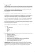
Growth and abnormal profitability reinforce each other:
, The median growth rate was 5% over the period 1968-2019. This holds for both companies that did
initially very good or bad; after some period, growth rates generally return to the 5% median. It is
questionable, however, whether this number also is a good estimate for the future when you make
forecasts. It would be better to base your arguments upon clear economics reasoning.
According to growth theory, the long-run growth rate for an economy is the long-run rate of
T
( Ro E t −r ) ∙C E t−1 ( Ro E∞ −r ) ∙C E T
technological change. P0=C E0 + E0
[ ∑
t =1 ( 1+r )t
+
( 1+ r )T ∙ ( r−g∞ ) ]
. The best guess for
the rate of technological change is 3-5%. If you take a larger growth rate, you basically assume that the
firm grows more than the economy forever, which is unrealistic.
In the case of Intel, investors’ expectations about large profitability and high growth rates interacted.
Investors extrapolated future sales growth too far into the future. Correction shave off a large bunk of
value.
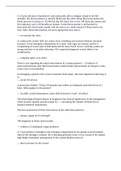
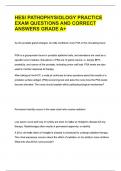
Firms with a high market-to-book
ratio are often called growth firms,
whereas firms with a low market-
to-book ratio are often called value
firms. The graph on the right shows
that growth firms generally react
stronger to earnings surprises than
value firms.
Takeaways:
Sales growth rates and gross margins are usually the most critical forecasting assumptions.
The economic value of the firm is the discounted sum of expected future cash flows. Economic value,
however, is not necessarily equal to market value.
The three steps of equity valuation:
1. Understanding the past
2. Forecasting the future
3. Valuation
What is the maximum you are willing to pay for an investment that you expect to yield EUR 100 for
three years while a comparable risky investment is expected to return 8% per year? Answer:
CF 1 CF 2 CF 3 100 100 100
V 0=Ε 0
[ ( 1+r ) 1
+
(1+r ) 2
+
( 1+ r ) 3
] [
=Ε + +
]
( 1+ 0.08 ) ( 1+0.08 ) ( 1+0.08 )3
1 2
=257.71.
The value of an equity interest is based on the present value of the expected future cash dividends to be
∞
DI V t
received: P0=E 0
[ ( )]
∑
t=1 ( 1+r )t
, where P0 is the value of the common equity at time 0, DIVt is the
amount of cash dividends to be paid in period t, r is the discount rate, and E0 [·] indicates that what’s
inside the brackets is uncertain (i.e., expected values). The dividend discount formula is rarely used
directly, because (1) dividends do not directly reflect performance (a firm can also pay out dividends
when it is making a loss), (2) dividends are to a large extent discretionary, and (3) many firms do not pay
dividend right now but promise to pay later.
Periodic return and re-investment:
, ∞
DI V t
Recall that P0=E 0
[ ( )]
∑
t=1 ( 1+r )t
. Generally, C E t =C E t−1 + N I t −DI V t (where CE is the book value of
common equity and NI is net income), so DI V t =N I t −ΔC E t . Plugging this into the first formula and
∞ ∞
N I t −r ∙C Et−1 ( Ro E t−r ) ∙ C E t−1
simplifying yields P0=C E0 + E0
[ ∑
t =1 ( 1+r )
t
]
=C E 0 + E0
[ ∑
t=1 ( 1+r )
t
] , where RoE
is the return on equity (NI / CE).
∞
( Ro E t −r ) ∙C E t−1
Direct inputs to P0=C E0 + E0
[ ∑
t =1 ( 1+r )
t
] are the core value drivers. We distinguish
investment growth (g), risk (r), and profitability (RoE).
Profitability
o Return on equity (RoE) is the key profitability measure. It is the Return on Investment
Earnings for the period
(RoI) for equity investors. RoI = .
Investment at thebeginning of the period
o RoE is the rate of return that equity owners get. RoE must be higher than the
opportunity cost (r) in order to generate value; only if RoE is greater than r, the firm
creates value. We call this opportunity cost (r) ‘expected return’ or ‘cost of equity
capital’.
o When looking at the RoE over time, we see that the mean RoE generally increased as of
1968, but then decreased again from about 1990 onwards. Next to that, its spread has
increased considerably over time. Business and accounting changes affected RoE.
Investment growth
o Besides profitability, the amount of capital invested is also crucial. Investment
depreciates and becomes obsolete: investments need to grow to expand the business,
and investments in new assets are needed to not become obsolete and to stay
competitive.
Risk
o It is quite difficult to forecast next year’s payoff because of a high degree of volatility.
Equity investing, relative to long-term Treasury bills, is therefore quite risky.
o Expected values are uncertain. To adjust for the uncertainty (riskiness) of expectations,
we discount them: r is our measure of this uncertainty. However, coming up with the
right (‘true’) discount rate, r, is challenging. You could use asset pricing models for this.
If we assume that profitability is constant, Ro Et +1=Ro E t =RoE , and capital grows by g each year,
C E t=( 1+ g ) C Et −1, then our basic earnings-based valuation formula simplifies a lot:
∞
( Ro E t −r ) ∙C E t−1 ( Ro E1−r ) ∙C E 0 ( Ro E 1−r ) ∙ ( 1+ g ) C E 0 ( Ro
P0=C E0 + E0
[ ∑
t =1 ( 1+r )
t
]=C E 0+ E0
[ ( 1+r )
1
+
( 1+r )
2
]
+ … =C E0 + E0 [
. You could also rewrite this formula such that the implied growth rate becomes the unknown variable
on the left-hand side of the formula. Then for several discount rates, you can tabulate the corresponding
growth rates.
,Lecture 2 (05-02-2021) – Practice Session
∞
( Ro E t −r ) ∙C E t−1
Direct inputs to P0=C E0 + E0
[ ∑
t =1 ( 1+r )
t
] are the core value drives. We have three value
drivers: growth (g), profitability (RoE), and risk (r). A profitability of 10% does not say that much. You
have to compare it with company’s cost of capital (which reflects the company’s riskiness); if that one is
also 10%, the company does not generate any value. But if it is 5%, the company generates value. If the
investment growth (g) changes, the cost of capital (r) is likely to change as well.
Earnings announcements are the single most important information event, both in terms of absolute
returns as well as share turnover. Those announcements in the third quarter are the most important
ones, because most firms first provide details on next year in the third quarter.
On September 21, 2000, Intel released an
earnings warning. On the right, you see what
has changed.
∞
( Ro E t −r ) ∙C E t−1
From the first lecture, we learned that P0=C E0 + E0
[ ∑
t =1 ( 1+r )
t
]
. The standard approach is
to forecast the first 20 years explicitly and afterwards assume a constant profitability and growth:
20
( Ro E t −r ) ∙C E t−1 ( Ro E∞ −r ) ∙C E 20
P0=C E0 + E0
[ ∑
t =1 ( 1+r )t
+
( 1+ r )20 ∙ ( r−g ∞ ) ] .
You make your assumptions based on an analysis of the business. The amount of sales is a very
important forecast, because many other items are calculated as a percentage of sales.
When we extrapolate unusually high sale growth far into the future, small revisions in sales growth can
have a huge impact on value. Remember that sales growth is rapidly mean reverting.
Growth and abnormal profitability reinforce each other:
, The median growth rate was 5% over the period 1968-2019. This holds for both companies that did
initially very good or bad; after some period, growth rates generally return to the 5% median. It is
questionable, however, whether this number also is a good estimate for the future when you make
forecasts. It would be better to base your arguments upon clear economics reasoning.
According to growth theory, the long-run growth rate for an economy is the long-run rate of
T
( Ro E t −r ) ∙C E t−1 ( Ro E∞ −r ) ∙C E T
technological change. P0=C E0 + E0
[ ∑
t =1 ( 1+r )t
+
( 1+ r )T ∙ ( r−g∞ ) ]
. The best guess for
the rate of technological change is 3-5%. If you take a larger growth rate, you basically assume that the
firm grows more than the economy forever, which is unrealistic.
In the case of Intel, investors’ expectations about large profitability and high growth rates interacted.
Investors extrapolated future sales growth too far into the future. Correction shave off a large bunk of
value.
Firms with a high market-to-book
ratio are often called growth firms,
whereas firms with a low market-
to-book ratio are often called value
firms. The graph on the right shows
that growth firms generally react
stronger to earnings surprises than
value firms.
Takeaways:
Sales growth rates and gross margins are usually the most critical forecasting assumptions.