ENGINEERING VIBRATION
Solution Manual – Engineering Vibration, 5th Edition (Daniel J.
Inman) – Complete Problem Solutions (Chapters 1–8)
Bonie314 Stuvia
,Problems and Solutions Section 1.1 (1.1 through 1.19)
h h h h h h h
1.1 The spring of Figure 1.2 is successively loaded with mass and the corresponding (static)
h h h h h h h h h h h h h
displacement is recorded below. Plot the data and calculate the spring's stiffness. Note
h h h h h h h h h h h h h
that the data contain some error. Also calculate the standard deviation.
h h h h h h h h h h h
m(kg) 10 11 12 13 14 15 16
x(m) 1.14 1.25 1.37 1.48 1.59 1.71 1.82
Solution:
Free-body diagram: h
From the free-body diagram and static
h h h h h
equilibrium:
h
kx
kx mg h h (g 9.81m/ s2)
h h h h
k k mg/ x
h h h
k
m i 86.164
n
mg
20
The sample standard deviation in
h h h h
computed stiffness is:
h h h
n
m 15 i1(k )2
i h
h h
h h h 0.164 h
n 1 h h
10
0 1 2
x
Plot of mass in kg versus displacement in m
h h h h h h h h
Computation of slope from mg/x h h h h
m(kg) x(m) k(N/m)
10 1.14 86.05
11 1.25 86.33
12 1.37 85.93
13 1.48 86.17
14 1.59 86.38
15 1.71 86.05
16 1.82 86.24
, 1.2 Derive the solution of m˙x˙ kx 0 and plot the result for at least two periods for the case
h h h h h h h h h h h h h h h h h h
with n = 2 rad/s, x0 = 1 mm, and v0 = 5 mm/s.
h h h h h h h h h h h
Solution:
Given:
m!x!kx 0 (1) h h
Assume: x(t) ae . Then: x! are and !x! ar e . Substitute into equation (1) to
rt h
2 rt h
rt
h h h h h h h h h h h
get:
h
mar2ert kaert 0 h h
mr2 k 0 h h
k
r hi h
m
Thus there are two solutions:
h h h h
k h h kh h
i ht h i t
x1 c1e h
m
h h , and h
2 c2 e h
m
h
h x
k
2 rad/s where n h h h h
m
The sum of x1 and x2 is also a solution so that the total solution is:
h h h h h h h h h h h h h h h
x x x c e2it c e2it
h h
h
h
h
1 2 1 2
Substitute initial conditions: x0 = 1 mm, v0 =
h h h h h h h h 5 mm/s
x0c1c2 x0 1 c2 1 c1, and v0x!02ic1 2ic2 v0 5 mm/s
h h h h h h h h h h h h h h h h h h
2c1 2c2 5 i. Combining the two underlined expressions (2 eqs in 2 unkowns):
h h h h h h h h h h h h h h h
1 5 1 5
2c 2 2c 5 i c i, and
h h h h h
h h h i h h h h h h h h
hc
1 1 1 2
2 4 2 4
Therefore the solution is: h h h
xe 1 5 i 2it 1 5 i e2it
h
h
h
h
h
h h h h
2 4
h
h
2 4 h
h h h
Using the Euler formula to evaluate the exponential terms yields:
h h h h h h h h h
1 5 1 5
i cos2t isin2t i cos2t isin2t
h h h h
x h
h
h
h
h h h h h
h
h
h
h h h h h h
2 4 2 4
h h h h
5 3
x(t) cos2t sin2t sin2t 0.7297
h h
h h h h h h h h h h
2 2
, Using Mathcad the plot is:
h h h h
5. h
x t
h h cos 2. t h sin 2. t
h
h
2
2
x t
h
0 5 10
2
t
Solution Manual – Engineering Vibration, 5th Edition (Daniel J.
Inman) – Complete Problem Solutions (Chapters 1–8)
Bonie314 Stuvia
,Problems and Solutions Section 1.1 (1.1 through 1.19)
h h h h h h h
1.1 The spring of Figure 1.2 is successively loaded with mass and the corresponding (static)
h h h h h h h h h h h h h
displacement is recorded below. Plot the data and calculate the spring's stiffness. Note
h h h h h h h h h h h h h
that the data contain some error. Also calculate the standard deviation.
h h h h h h h h h h h
m(kg) 10 11 12 13 14 15 16
x(m) 1.14 1.25 1.37 1.48 1.59 1.71 1.82
Solution:
Free-body diagram: h
From the free-body diagram and static
h h h h h
equilibrium:
h
kx
kx mg h h (g 9.81m/ s2)
h h h h
k k mg/ x
h h h
k
m i 86.164
n
mg
20
The sample standard deviation in
h h h h
computed stiffness is:
h h h
n
m 15 i1(k )2
i h
h h
h h h 0.164 h
n 1 h h
10
0 1 2
x
Plot of mass in kg versus displacement in m
h h h h h h h h
Computation of slope from mg/x h h h h
m(kg) x(m) k(N/m)
10 1.14 86.05
11 1.25 86.33
12 1.37 85.93
13 1.48 86.17
14 1.59 86.38
15 1.71 86.05
16 1.82 86.24
, 1.2 Derive the solution of m˙x˙ kx 0 and plot the result for at least two periods for the case
h h h h h h h h h h h h h h h h h h
with n = 2 rad/s, x0 = 1 mm, and v0 = 5 mm/s.
h h h h h h h h h h h
Solution:
Given:
m!x!kx 0 (1) h h
Assume: x(t) ae . Then: x! are and !x! ar e . Substitute into equation (1) to
rt h
2 rt h
rt
h h h h h h h h h h h
get:
h
mar2ert kaert 0 h h
mr2 k 0 h h
k
r hi h
m
Thus there are two solutions:
h h h h
k h h kh h
i ht h i t
x1 c1e h
m
h h , and h
2 c2 e h
m
h
h x
k
2 rad/s where n h h h h
m
The sum of x1 and x2 is also a solution so that the total solution is:
h h h h h h h h h h h h h h h
x x x c e2it c e2it
h h
h
h
h
1 2 1 2
Substitute initial conditions: x0 = 1 mm, v0 =
h h h h h h h h 5 mm/s
x0c1c2 x0 1 c2 1 c1, and v0x!02ic1 2ic2 v0 5 mm/s
h h h h h h h h h h h h h h h h h h
2c1 2c2 5 i. Combining the two underlined expressions (2 eqs in 2 unkowns):
h h h h h h h h h h h h h h h
1 5 1 5
2c 2 2c 5 i c i, and
h h h h h
h h h i h h h h h h h h
hc
1 1 1 2
2 4 2 4
Therefore the solution is: h h h
xe 1 5 i 2it 1 5 i e2it
h
h
h
h
h
h h h h
2 4
h
h
2 4 h
h h h
Using the Euler formula to evaluate the exponential terms yields:
h h h h h h h h h
1 5 1 5
i cos2t isin2t i cos2t isin2t
h h h h
x h
h
h
h
h h h h h
h
h
h
h h h h h h
2 4 2 4
h h h h
5 3
x(t) cos2t sin2t sin2t 0.7297
h h
h h h h h h h h h h
2 2
, Using Mathcad the plot is:
h h h h
5. h
x t
h h cos 2. t h sin 2. t
h
h
2
2
x t
h
0 5 10
2
t