Statistics 2
VU Amsterdam, Year 2, Period 4
How to use this summary:
Each chapters discussed together are linked to the same lecture
After two lectures (a week) there is a space to write a very short summary
Use the sidebar with cues of topics and terms to
study by covering the actual content next to it
(If you want, you can also add your own cues)
Chapter 2 & 3
Here you can read what the chapter(s) are about
Blue highlights Green highlights are for structuring
indicate a topic 1. Terms can also be highlighted in the text
2. Sometimes, if an explanation is a bit longer (or you want to scan the text),
a pink highlight might be used again to give structure to the text and
Yellow highlights highlight the most important aspects of the text.
indicate a term
, Lecture 1: Recap of Stat 1 ch. 1-4
Measurement levels of variables, descriptive statistics & probability distributions
/
What is a variable? A variable is a characteristic that can vary in value among subjects in a sample
or a population. They each have their own measurement level, which
determines the statistical method that is to be used.
Measurement levels 1. Nominal
2. Ordinal
unordered, only has the quality of identity)
has the qualities of identity and order) } categorical
3. Interval
4. Ratio
identity, order and quantity in equal units)
identity, order, quantity and an absolute zero point) } nfuetarniitative
Parametric methods = suitable for interval and ratio (quantitative) data (quantitative y )
Nonparametric met. = suitable for nominal and ordinal (categorical) data ( categorical y)
Descriptive statistics = used to summarize data with tables and figures
We can - summarize per one variable (distribution)
:÷÷÷÷÷:
- summarize multiple variables (associations)
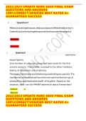
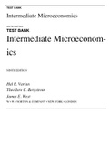
Categorical data Descriptive statistics for categorical data = frequencies and bar graphs
" "
.÷÷÷÷÷÷÷÷÷÷÷÷
:
.
Quantitative data Descriptive statistics for quantitative data = frequencies and histograms
Now the bars are
o_0
M
connected because
§
they cover a
range
of values
Fon!f¥asd
in a
continuous way
categories
,Steam-and-leafplots For quantitative data, you can also express these in steam-and-leafplots.
The consequent histogram is then turned.
µ÷
↳
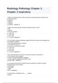
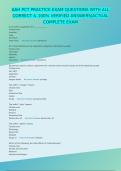
Graph descriptions
(& examples)
Good
to Be ed
Bell-shaped U-shaped Positive skew Negative skew
(intelligence) (extreme politics) (psychopathology) (happiness)
Data centre: Mean, Mean = the average Median = the middle nr. Mode = the most frequent nr.
median, mode
. . ..
.. . .. .
.÷÷÷÷ .
Data variability:
Range = the difference between the minimum and maximum variable
Deviation = the difference from the mean for each item
(yi -
51 Yi = item score
4- mean y =
Sum of Squares = 1. Squaring the deviation score for each item (to eliminate negative numbers)
2. Summing these all up —> shows the total deviance from the mean
E
'
{ fyi -
y)
=
sum
Z
gets rid of
negatives
Variance 5) = the standardized sum of squares
{ ( yi -
512 : n -
I = Standardisation
n -
7
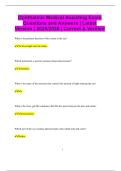
SD ( s ) = gives the average deviation from the mean (through cancelling out the square)
ECyi.TK ✓ 2
cancels out the
n -
I
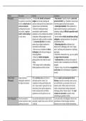
, From histogram 1 -
Yi -
5
•
to SD same thing - 2 .
Square that
f÷
8-D
3 .
Sum
u .
Standardize
( : n -
T )
5. Take the
root N
t
mean
= 5
The empirical rule
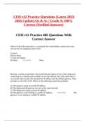
Measures of position A boxplot devides the date up in four equal parts called quartiles
""""" "" "
"
"
"
"
"
quartile or
: ÷:÷ ÷ ÷
1501 .
of data)
.
above the 3rd Id
Probability (p) = the chance that an observation takes on a particular value
—> Each possible value of a variable has a specific probability of occurring
—> This is represented in a probability distribution = all possible values
of a variable and their probabilities
Discrete vs cont. Discrete distributions
- Each value has a probability
:- Represented in a histogram
Continuous distributions
- Infinite number or possible values, probability given to intervals
:- Represented in the area under the curve
VU Amsterdam, Year 2, Period 4
How to use this summary:
Each chapters discussed together are linked to the same lecture
After two lectures (a week) there is a space to write a very short summary
Use the sidebar with cues of topics and terms to
study by covering the actual content next to it
(If you want, you can also add your own cues)
Chapter 2 & 3
Here you can read what the chapter(s) are about
Blue highlights Green highlights are for structuring
indicate a topic 1. Terms can also be highlighted in the text
2. Sometimes, if an explanation is a bit longer (or you want to scan the text),
a pink highlight might be used again to give structure to the text and
Yellow highlights highlight the most important aspects of the text.
indicate a term
, Lecture 1: Recap of Stat 1 ch. 1-4
Measurement levels of variables, descriptive statistics & probability distributions
/
What is a variable? A variable is a characteristic that can vary in value among subjects in a sample
or a population. They each have their own measurement level, which
determines the statistical method that is to be used.
Measurement levels 1. Nominal
2. Ordinal
unordered, only has the quality of identity)
has the qualities of identity and order) } categorical
3. Interval
4. Ratio
identity, order and quantity in equal units)
identity, order, quantity and an absolute zero point) } nfuetarniitative
Parametric methods = suitable for interval and ratio (quantitative) data (quantitative y )
Nonparametric met. = suitable for nominal and ordinal (categorical) data ( categorical y)
Descriptive statistics = used to summarize data with tables and figures
We can - summarize per one variable (distribution)
:÷÷÷÷÷:
- summarize multiple variables (associations)
Categorical data Descriptive statistics for categorical data = frequencies and bar graphs
" "
.÷÷÷÷÷÷÷÷÷÷÷÷
:
.
Quantitative data Descriptive statistics for quantitative data = frequencies and histograms
Now the bars are
o_0
M
connected because
§
they cover a
range
of values
Fon!f¥asd
in a
continuous way
categories
,Steam-and-leafplots For quantitative data, you can also express these in steam-and-leafplots.
The consequent histogram is then turned.
µ÷
↳
Graph descriptions
(& examples)
Good
to Be ed
Bell-shaped U-shaped Positive skew Negative skew
(intelligence) (extreme politics) (psychopathology) (happiness)
Data centre: Mean, Mean = the average Median = the middle nr. Mode = the most frequent nr.
median, mode
. . ..
.. . .. .
.÷÷÷÷ .
Data variability:
Range = the difference between the minimum and maximum variable
Deviation = the difference from the mean for each item
(yi -
51 Yi = item score
4- mean y =
Sum of Squares = 1. Squaring the deviation score for each item (to eliminate negative numbers)
2. Summing these all up —> shows the total deviance from the mean
E
'
{ fyi -
y)
=
sum
Z
gets rid of
negatives
Variance 5) = the standardized sum of squares
{ ( yi -
512 : n -
I = Standardisation
n -
7
SD ( s ) = gives the average deviation from the mean (through cancelling out the square)
ECyi.TK ✓ 2
cancels out the
n -
I
, From histogram 1 -
Yi -
5
•
to SD same thing - 2 .
Square that
f÷
8-D
3 .
Sum
u .
Standardize
( : n -
T )
5. Take the
root N
t
mean
= 5
The empirical rule
Measures of position A boxplot devides the date up in four equal parts called quartiles
""""" "" "
"
"
"
"
"
quartile or
: ÷:÷ ÷ ÷
1501 .
of data)
.
above the 3rd Id
Probability (p) = the chance that an observation takes on a particular value
—> Each possible value of a variable has a specific probability of occurring
—> This is represented in a probability distribution = all possible values
of a variable and their probabilities
Discrete vs cont. Discrete distributions
- Each value has a probability
:- Represented in a histogram
Continuous distributions
- Infinite number or possible values, probability given to intervals
:- Represented in the area under the curve