Blok 7 - BK2103 Onderzoeksproject
Overview block 6
Concepts and constructs vary based on their degree of abstractness: a concept is more abstract
than a construct.
Concept: communication skill (more abstract)
Construct: vocabulary and syntax skill (less abstract)
Importantly, concepts and construct are both abstract entities, they are not directly
measurable. The operationalization of a concept/construct is called “variable”.
Challenge 1: Levels of measurement: nominal, ordinal, interval, ratio.
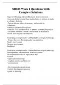
In the data base, we have one item = one column
First, we check the scale’s reliability with Cronbach alpha
Participant BR1 BR2 BR3 BR4
Romain 5 5 6 6
Jenny 4 4 4 5
….
Zoe 3 2 3 4
If a<-0.70, then you may compute the composite measure.
If a >0.70, then you may delete one or several items until a >-0.70
If a <--0.70, for a 3-items combination (e.g., BR1, BR2, BR3) then use, if not
If a >-0.70 for a 2-item combination (e.g., BR1, BR2) etc.
Reverse coded items: with a negative vs positive question. Recode the values from 1 to 7, new:
7 to 1. If the items are not on the same scale. On from 1-7 other from 1-5. Rescale the items. If
there is a mix between nominal and interval it is not possible to merge.
Researcher often label their several “theoretical” hypotheses in the following way:
H1: ease of use positively influences technology adoption
H2: innovativeness positively influence technology adoption
H3: age negatively influences technology adoption
For each of these “theoretical” hypotheses, we can associate two “statistical” hypotheses
known as null vs. alternative.
When the null vs. alternative are noted as H0 and H1, we could have a confusion
between the H1 (theoretical) and H1 (statistical)
Therefore, and from now on, we will use the following notations for the null (H0) and
alternative (Ha) hypothesis
Researcher Smith posits the following (theoretical) hypothesis
H1: variable X positively influences variable Y
Associated statistical hypotheses
H0: r <- 0
1
, H1: r > 0
General rules for: statistical: interpretation: if noted otherwise, risk level a = 0.05
If p <0.05, the researcher “rejects” the null hypothesis
If p >0.05, the researcher cannot “reject” the null hypothesis
General rules theoretical interpretation: if not noted otherwise, risk level a=0.05
If p<0.05 the results confirm (corroborates, validates) the researcher’s hypothesis
If p>0.05 the results do not confirm (corroborate, validate) the researcher’s hypothesis
In almost all research reports, researchers do not report the null/alternative (statistical)
hypothesis and whether it was rejected. Usually, researchers only mention whether the
(theoretical) hypothesis was confirmed/corroborated/validated, or not.
Example: research smith posits the following hypothesis.
H1: variable X positively influences variable Y
H2: variable W positively influences variable Y
“Results from statistical analyses show that the correlation coefficient between X and Y was
positive (r=0.21) and significant (r=0.19) and significant (p=0.01). H1 is validated.”
“Results from statistical analyses showed that the correlation coefficient between W and Y was
positive yet not yet significant (r=0.19, p=0.56). These results do not confirm H2.
Correlation
Correlation coefficient know as “Pearson’s R” can be sometimes noted with the Greek letter
p(ro). Not to be confused with the letter p, representing the p-value. Example:
H1: ease of use positively influences technology adoption
H0: r <- 0
Ha: r > 0
The results from the statistical analyses are r: 0.21, p=0.01. The results confirm the researcher’s
hypothesis.
T-Test
2
,ANOVA
Lecture 2
Correlation vs. causation
Causal inference is difficult. It does not always mean de variable causes the other one.
Correlation does not imply causation.
Example: why is shoe size related to reading ability?
Kids and adults, so age.
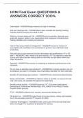
Several reasons why X and Y can correlate:
X causes Y
3
, Z causes X and Y
Spurious correlation (age in example)
Y causes X
Reverse causality: X appears to cause Y, but it is actually Y that causes Y.
Examples: Diversification and profitability, diversified firms tend to profit more.
-> This may be because more profitable firms need to find ways to to invest profits rather than
because diversification causes profitability.
Sales of a brand of soda are higher during weeks of heavy advertising.
The heavy advertising is done during periods of high consumption.
Third variable: X appears to cause Y, but both X and Y are actually caused by Z.
On the average, the more toys a child has, the higher his or her IQ.
Both the number of toys and IQ may be caused by family resources such as income.
On average, students who sit in the front of the class end up with higher grades.
However, students choose where they sit. Motivation may influence both sitting and grades.
When can we infer that X causes Y?
Three conditions for causality:
Relationship between X and Y: X and Y vary together
Time order: X cannot happen after Y
Elimination of other possible causal factors: all other possible causes held constant or
controlled
Basic features of a between-subjects design:
Independent variable that is ‘manipulated’ across group between-subject
Between-subject: one participant is assigned to one experimental condition of the IV
Within-subject: one participant is assigned to several experimental conditions
Dependent variable that is measured
Context: laboratory, online survey, field etc.
Controlling extraneous factors
All things but the independent variable are the same
Participants randomly assigned to groups
Measurement of other variables for statistical control
IV is always nominal. DV most of the time interval.
Example A: framing coupons
Framing: exposing the same information in a positive or negative way.
4
Overview block 6
Concepts and constructs vary based on their degree of abstractness: a concept is more abstract
than a construct.
Concept: communication skill (more abstract)
Construct: vocabulary and syntax skill (less abstract)
Importantly, concepts and construct are both abstract entities, they are not directly
measurable. The operationalization of a concept/construct is called “variable”.
Challenge 1: Levels of measurement: nominal, ordinal, interval, ratio.
In the data base, we have one item = one column
First, we check the scale’s reliability with Cronbach alpha
Participant BR1 BR2 BR3 BR4
Romain 5 5 6 6
Jenny 4 4 4 5
….
Zoe 3 2 3 4
If a<-0.70, then you may compute the composite measure.
If a >0.70, then you may delete one or several items until a >-0.70
If a <--0.70, for a 3-items combination (e.g., BR1, BR2, BR3) then use, if not
If a >-0.70 for a 2-item combination (e.g., BR1, BR2) etc.
Reverse coded items: with a negative vs positive question. Recode the values from 1 to 7, new:
7 to 1. If the items are not on the same scale. On from 1-7 other from 1-5. Rescale the items. If
there is a mix between nominal and interval it is not possible to merge.
Researcher often label their several “theoretical” hypotheses in the following way:
H1: ease of use positively influences technology adoption
H2: innovativeness positively influence technology adoption
H3: age negatively influences technology adoption
For each of these “theoretical” hypotheses, we can associate two “statistical” hypotheses
known as null vs. alternative.
When the null vs. alternative are noted as H0 and H1, we could have a confusion
between the H1 (theoretical) and H1 (statistical)
Therefore, and from now on, we will use the following notations for the null (H0) and
alternative (Ha) hypothesis
Researcher Smith posits the following (theoretical) hypothesis
H1: variable X positively influences variable Y
Associated statistical hypotheses
H0: r <- 0
1
, H1: r > 0
General rules for: statistical: interpretation: if noted otherwise, risk level a = 0.05
If p <0.05, the researcher “rejects” the null hypothesis
If p >0.05, the researcher cannot “reject” the null hypothesis
General rules theoretical interpretation: if not noted otherwise, risk level a=0.05
If p<0.05 the results confirm (corroborates, validates) the researcher’s hypothesis
If p>0.05 the results do not confirm (corroborate, validate) the researcher’s hypothesis
In almost all research reports, researchers do not report the null/alternative (statistical)
hypothesis and whether it was rejected. Usually, researchers only mention whether the
(theoretical) hypothesis was confirmed/corroborated/validated, or not.
Example: research smith posits the following hypothesis.
H1: variable X positively influences variable Y
H2: variable W positively influences variable Y
“Results from statistical analyses show that the correlation coefficient between X and Y was
positive (r=0.21) and significant (r=0.19) and significant (p=0.01). H1 is validated.”
“Results from statistical analyses showed that the correlation coefficient between W and Y was
positive yet not yet significant (r=0.19, p=0.56). These results do not confirm H2.
Correlation
Correlation coefficient know as “Pearson’s R” can be sometimes noted with the Greek letter
p(ro). Not to be confused with the letter p, representing the p-value. Example:
H1: ease of use positively influences technology adoption
H0: r <- 0
Ha: r > 0
The results from the statistical analyses are r: 0.21, p=0.01. The results confirm the researcher’s
hypothesis.
T-Test
2
,ANOVA
Lecture 2
Correlation vs. causation
Causal inference is difficult. It does not always mean de variable causes the other one.
Correlation does not imply causation.
Example: why is shoe size related to reading ability?
Kids and adults, so age.
Several reasons why X and Y can correlate:
X causes Y
3
, Z causes X and Y
Spurious correlation (age in example)
Y causes X
Reverse causality: X appears to cause Y, but it is actually Y that causes Y.
Examples: Diversification and profitability, diversified firms tend to profit more.
-> This may be because more profitable firms need to find ways to to invest profits rather than
because diversification causes profitability.
Sales of a brand of soda are higher during weeks of heavy advertising.
The heavy advertising is done during periods of high consumption.
Third variable: X appears to cause Y, but both X and Y are actually caused by Z.
On the average, the more toys a child has, the higher his or her IQ.
Both the number of toys and IQ may be caused by family resources such as income.
On average, students who sit in the front of the class end up with higher grades.
However, students choose where they sit. Motivation may influence both sitting and grades.
When can we infer that X causes Y?
Three conditions for causality:
Relationship between X and Y: X and Y vary together
Time order: X cannot happen after Y
Elimination of other possible causal factors: all other possible causes held constant or
controlled
Basic features of a between-subjects design:
Independent variable that is ‘manipulated’ across group between-subject
Between-subject: one participant is assigned to one experimental condition of the IV
Within-subject: one participant is assigned to several experimental conditions
Dependent variable that is measured
Context: laboratory, online survey, field etc.
Controlling extraneous factors
All things but the independent variable are the same
Participants randomly assigned to groups
Measurement of other variables for statistical control
IV is always nominal. DV most of the time interval.
Example A: framing coupons
Framing: exposing the same information in a positive or negative way.
4