COSC 3P03: Algorithms
The Complete Exam Survival Guide
Comprehensive Review with Solved Examples for Every Topic
1 Study Roadmap: Topics & Dependencies
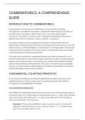
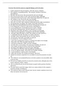
Use this flowchart to visualize how the course topics build upon each other.
Foundations
(Wk 1-2)
Asymptotic Analysis
Data Structures
Recursion (Wk 3)
Master Theorem
Recursion Trees
Dynamic Pro-
gramming (Wk 6)
Overlapping
Subproblems
Divide & Con- Ex: LCS, Subset Sum Greedy Algs (Wk 7)
quer (Wk 5) Local Optimality
Splitting & Merging Ex: Huffman
Ex: Closest Pair
Sorting (Wk 4) Graph Algs (Wk 8-9)
Linear Sorts Traversals, MST
Lower Bounds Shortest Paths
Complexity (Wk 11)
P vs NP Max Flow (Wk 10)
Reductions Flow Networks
Min-Cut
1
,2 Foundations: Analysis & Recursion
2.1 How Asymptotic Analysis Works
We analyze algorithms by bounding their running time functions, f (n), using simpler functions, g(n), as n → ∞.
We ignore constants because they depend on hardware, not the algorithm logic.
Visualizing Growth Rates
• Big-O (O): ”Less than or equal to”. f (n) ≤ c · g(n) for large n. (Worst Case).
• Big-Omega (Ω): ”Greater than or equal to”. f (n) ≥ c · g(n) for large n. (Best Case / Lower Bound).
• Theta (Θ): ”Equal to”. The function is sandwiched between c1 · g(n) and c2 · g(n).
Solved Example: Comparing Functions
Question: Compare f (n) = n2 − 3n and g(n) = 2n2 .
Solution: We check the limit limn→∞ fg(n)
(n)
.
n2 − 3n 1 3 1
lim 2
= lim ( − )=
n→∞ 2n n→∞ 2 2n 2
Since the limit is a positive constant (0 < 1/2 < ∞), f (n) = Θ(g(n)). They grow at the same rate.
2.2 How Recursion Trees Work
Recursion trees allow us to visualize the total work of a divide-and-conquer algorithm by summing work across all
levels.
The 3 Cases of Tree Summation
Consider T (n) = rT (n/c) + f (n).
1. Root Dominated (f (n) is heavy): The work at the root is huge compared to the children. Total
time ≈ O(f (n)).
2. Balanced (Equal work): Every level has roughly the same total work. Total time ≈ f (n) × Height.
(e.g., Merge Sort).
3. Leaf Dominated (Many children): The number of subproblems grows so fast that the leaves account
for most of the work. Total time ≈ Number of Leaves.
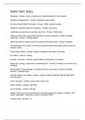
Solved Example: Recurrence Tree Analysis
Problem: Solve T (n) = 2T (n/2) + n2 .
Tree Construction:
• Level 0: 1 node of cost n2 . Total: n2 .
• Level 1: 2 nodes of cost (n/2)2 = n2 /4. Total: 2 × n2 /4 = n2 /2.
• Level 2: 4 nodes of cost (n/4)2 = n2 /16. Total: 4 × n2 /16 = n2 /4.
Analysis: The total work is n2 (1 + 1/2 + 1/4 + . . . ). This is a geometric series that sums to 2n2 .
Result: T (n) = Θ(n2 ). (Root Dominated).
2
,2.2.1 Example: Peasant Multiplication
Mechanism: To calculate x · y, we halve x and double y until x = 0. If x is odd, we add the current y to the
result.
Solved Example: Peasant Multiplication
Multiply: 13 × 11.
x (Halve) y (Double) Add to Prod?
13 11 Yes (+11)
6 22 No
3 44 Yes (+44)
1 88 Yes (+88)
Total: 11 + 44 + 88 = 143.
Complexity: Depth is log2 13 ≈ 3. Time O(log x).
3 Sorting: Mechanics & Bounds
3.1 Why Comparison Sorts are Limited
Comparison sorts can distinguish between input permutations only by comparing two elements at a time.
The Adversary Argument (Lower Bound)
Imagine an ”Adversary” who wants to force your algorithm to do maximum work.
1. You ask: ”Is ai < aj ?”
2. The Adversary gives an answer that keeps the maximum number of possible sorted permutations alive.
3. To distinguish between n! permutations, you need a tree of height log2 (n!).
4. Using Stirling’s approximation, log2 (n!) ≈ n log n − 1.44n.
5. Therefore, no comparison sort can be faster than Ω(n log n).
3.2 How Linear Sorts Cheat the Bound
Linear sorts (Counting, Radix) avoid comparisons by using the actual values of the numbers to determine
position.
3.2.1 Counting Sort Mechanism
To sort array A with values in range [0, k]:
1. Frequency Array: Create array C[0..k]. Iterate A, incrementing C[A[i]] for each element.
2. Accumulate: Modify C such that C[i] = C[i] + C[i − 1]. Now C[x] tells us exactly how many elements are
≤ x.
3. Place: Iterate A backwards. Place element A[i] into output array B at index C[A[i]]. Decrement C[A[i]].
3
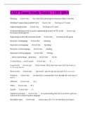
, Visualizing Counting Sort: A = [2, 5, 3, 0, 2, 3, 0, 3]
Step 1: Input Array A (Indices 1-8)
Index 1 2 3 4 5 6 7 8
A 2 5 3 0 2 3 0 3
Step 2: Frequency Array C (Count occurrences)
Index 0 1 2 3 4 5
Count 2 0 2 3 0 1
(e.g., ’0’ appears 2 times, ’3’ appears 3 times)
Step 3: Accumulate Array C (C[i] = C[i] + C[i − 1])
Index 0 1 2 3 4 5
Logic 2 2+0 2+2 4+3 7+0 7+1
Value 2 2 4 7 7 8
(This tells us the last position of each number in the sorted array)
Step 4: Final Output Array B
Index 1 2 3 4 5 6 7 8
B 0 0 2 2 3 3 3 5
4 Geometry & Lower Bound Reductions
4.1 Finding the Maximum
Problem: Find the maximum element in a list A of size n.
Algorithm: Scan the list, keeping track of the max seen so far.
Comparison Bound: To find the max, every element except the winner must ”lose” at least one comparison.
Therefore, we need at least n − 1 comparisons.
Lower Bound: Ω(n).
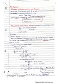
Tournament Method Visualization
To prove optimality or find max and min together efficiently.
Max(8)
Max(8) Max(7)
Max(8) Max(5) Max(7) Max(4)
3 8 2 5 7 1 4 0
Logic: Pairwise comparisons build a tournament tree. The root is the global max.
4.2 Convex Hull
Definition: The smallest convex polygon containing all points in a set S. Think of it as a rubber band stretched
around nails.
4
The Complete Exam Survival Guide
Comprehensive Review with Solved Examples for Every Topic
1 Study Roadmap: Topics & Dependencies
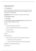
Use this flowchart to visualize how the course topics build upon each other.
Foundations
(Wk 1-2)
Asymptotic Analysis
Data Structures
Recursion (Wk 3)
Master Theorem
Recursion Trees
Dynamic Pro-
gramming (Wk 6)
Overlapping
Subproblems
Divide & Con- Ex: LCS, Subset Sum Greedy Algs (Wk 7)
quer (Wk 5) Local Optimality
Splitting & Merging Ex: Huffman
Ex: Closest Pair
Sorting (Wk 4) Graph Algs (Wk 8-9)
Linear Sorts Traversals, MST
Lower Bounds Shortest Paths
Complexity (Wk 11)
P vs NP Max Flow (Wk 10)
Reductions Flow Networks
Min-Cut
1
,2 Foundations: Analysis & Recursion
2.1 How Asymptotic Analysis Works
We analyze algorithms by bounding their running time functions, f (n), using simpler functions, g(n), as n → ∞.
We ignore constants because they depend on hardware, not the algorithm logic.
Visualizing Growth Rates
• Big-O (O): ”Less than or equal to”. f (n) ≤ c · g(n) for large n. (Worst Case).
• Big-Omega (Ω): ”Greater than or equal to”. f (n) ≥ c · g(n) for large n. (Best Case / Lower Bound).
• Theta (Θ): ”Equal to”. The function is sandwiched between c1 · g(n) and c2 · g(n).
Solved Example: Comparing Functions
Question: Compare f (n) = n2 − 3n and g(n) = 2n2 .
Solution: We check the limit limn→∞ fg(n)
(n)
.
n2 − 3n 1 3 1
lim 2
= lim ( − )=
n→∞ 2n n→∞ 2 2n 2
Since the limit is a positive constant (0 < 1/2 < ∞), f (n) = Θ(g(n)). They grow at the same rate.
2.2 How Recursion Trees Work
Recursion trees allow us to visualize the total work of a divide-and-conquer algorithm by summing work across all
levels.
The 3 Cases of Tree Summation
Consider T (n) = rT (n/c) + f (n).
1. Root Dominated (f (n) is heavy): The work at the root is huge compared to the children. Total
time ≈ O(f (n)).
2. Balanced (Equal work): Every level has roughly the same total work. Total time ≈ f (n) × Height.
(e.g., Merge Sort).
3. Leaf Dominated (Many children): The number of subproblems grows so fast that the leaves account
for most of the work. Total time ≈ Number of Leaves.
Solved Example: Recurrence Tree Analysis
Problem: Solve T (n) = 2T (n/2) + n2 .
Tree Construction:
• Level 0: 1 node of cost n2 . Total: n2 .
• Level 1: 2 nodes of cost (n/2)2 = n2 /4. Total: 2 × n2 /4 = n2 /2.
• Level 2: 4 nodes of cost (n/4)2 = n2 /16. Total: 4 × n2 /16 = n2 /4.
Analysis: The total work is n2 (1 + 1/2 + 1/4 + . . . ). This is a geometric series that sums to 2n2 .
Result: T (n) = Θ(n2 ). (Root Dominated).
2
,2.2.1 Example: Peasant Multiplication
Mechanism: To calculate x · y, we halve x and double y until x = 0. If x is odd, we add the current y to the
result.
Solved Example: Peasant Multiplication
Multiply: 13 × 11.
x (Halve) y (Double) Add to Prod?
13 11 Yes (+11)
6 22 No
3 44 Yes (+44)
1 88 Yes (+88)
Total: 11 + 44 + 88 = 143.
Complexity: Depth is log2 13 ≈ 3. Time O(log x).
3 Sorting: Mechanics & Bounds
3.1 Why Comparison Sorts are Limited
Comparison sorts can distinguish between input permutations only by comparing two elements at a time.
The Adversary Argument (Lower Bound)
Imagine an ”Adversary” who wants to force your algorithm to do maximum work.
1. You ask: ”Is ai < aj ?”
2. The Adversary gives an answer that keeps the maximum number of possible sorted permutations alive.
3. To distinguish between n! permutations, you need a tree of height log2 (n!).
4. Using Stirling’s approximation, log2 (n!) ≈ n log n − 1.44n.
5. Therefore, no comparison sort can be faster than Ω(n log n).
3.2 How Linear Sorts Cheat the Bound
Linear sorts (Counting, Radix) avoid comparisons by using the actual values of the numbers to determine
position.
3.2.1 Counting Sort Mechanism
To sort array A with values in range [0, k]:
1. Frequency Array: Create array C[0..k]. Iterate A, incrementing C[A[i]] for each element.
2. Accumulate: Modify C such that C[i] = C[i] + C[i − 1]. Now C[x] tells us exactly how many elements are
≤ x.
3. Place: Iterate A backwards. Place element A[i] into output array B at index C[A[i]]. Decrement C[A[i]].
3
, Visualizing Counting Sort: A = [2, 5, 3, 0, 2, 3, 0, 3]
Step 1: Input Array A (Indices 1-8)
Index 1 2 3 4 5 6 7 8
A 2 5 3 0 2 3 0 3
Step 2: Frequency Array C (Count occurrences)
Index 0 1 2 3 4 5
Count 2 0 2 3 0 1
(e.g., ’0’ appears 2 times, ’3’ appears 3 times)
Step 3: Accumulate Array C (C[i] = C[i] + C[i − 1])
Index 0 1 2 3 4 5
Logic 2 2+0 2+2 4+3 7+0 7+1
Value 2 2 4 7 7 8
(This tells us the last position of each number in the sorted array)
Step 4: Final Output Array B
Index 1 2 3 4 5 6 7 8
B 0 0 2 2 3 3 3 5
4 Geometry & Lower Bound Reductions
4.1 Finding the Maximum
Problem: Find the maximum element in a list A of size n.
Algorithm: Scan the list, keeping track of the max seen so far.
Comparison Bound: To find the max, every element except the winner must ”lose” at least one comparison.
Therefore, we need at least n − 1 comparisons.
Lower Bound: Ω(n).
Tournament Method Visualization
To prove optimality or find max and min together efficiently.
Max(8)
Max(8) Max(7)
Max(8) Max(5) Max(7) Max(4)
3 8 2 5 7 1 4 0
Logic: Pairwise comparisons build a tournament tree. The root is the global max.
4.2 Convex Hull
Definition: The smallest convex polygon containing all points in a set S. Think of it as a rubber band stretched
around nails.
4