PROBLEM 1.1
KNOWN: Temperature distribution in wall of Example 1.1.
FIND: Heat fluxes and heat rates at x = 0 and x = L.
SCHEMATIC:
ASSUMPTIONS: (1) One-dimensional conduction through the wall, (2) constant thermal conductivity,
(3) no internal thermal energy generation within the wall.
PROPERTIES: Thermal conductivity of wall (given): k = 1.7 W/m·K.
ANALYSIS: The heat flux in the wall is by conduction and is described by Fourier’s law,
dT
q′′x = −k (1)
dx
Since the temperature distribution is T(x) = a + bx, the temperature gradient is
dT
=b (2)
dx
Hence, the heat flux is constant throughout the wall, and is
dT
q′′x =−k =−kb =−1.7 W/m ⋅ K × ( −1000 K/m ) =1700 W/m 2 <
dx
Since the cross-sectional area through which heat is conducted is constant, the heat rate is constant and is
qx =q′′x × (W × H ) =1700 W/m 2 × (1.2 m × 0.5 m ) =1020 W <
Because the heat rate into the wall is equal to the heat rate out of the wall, steady-state conditions exist. <
COMMENTS: (1) If the heat rates were not equal, the internal energy of the wall would be changing
with time. (2) The temperatures of the wall surfaces are T 1 = 1400 K and T 2 = 1250 K.
, PROBLEM 1.2
KNOWN: Thermal conductivity, thickness and temperature difference across a sheet of rigid
extruded insulation.
FIND: (a) The heat flux through a 3 m × 3 m sheet of the insulation, (b) the heat rate through
the sheet, and (c) the thermal conduction resistance of the sheet.
SCHEMATIC:
m22
A = 49m
k = 0.029
qcond
12 °C
T1 – T2 = 10˚C
T1 T2
25 mm
L = 20
x
ASSUMPTIONS: (1) One-dimensional conduction in the x-direction, (2) Steady-state
conditions, (3) Constant properties.
ANALYSIS: (a) From Equation 1.2 the heat flux is
dT T -T W 12 K W
q′′x = -k = k 1 2 = 0.029 × = 13.9 2 <
dx L m⋅K 0.025 m m
(b) The heat rate is
W
q x = q′′x ⋅ A = 13.9 2
× 9 m 2 = 125 W <
m
(c) From Eq. 1.11, the thermal resistance is
R t,cond =
∆T / q x = 12 K /125 W =
0.096 K/W <
COMMENTS: (1) Be sure to keep in mind the important distinction between the heat flux
(W/m2) and the heat rate (W). (2) The direction of heat flow is from hot to cold. (3) Note that
a temperature difference may be expressed in kelvins or degrees Celsius. (4) The conduction
thermal resistance for a plane wall could equivalently be calculated from R t,cond = L/kA.
, PROBLEM 1.3
KNOWN: Thickness and thermal conductivity of a wall. Heat flux applied to one face and
temperatures of both surfaces.
FIND: Whether steady-state conditions exist.
SCHEMATIC:
L = 10 mm
T2 = 30°C
q” = 20 W/m2
q″cond
T1 = 50°C k = 12 W/m∙K
ASSUMPTIONS: (1) One-dimensional conduction, (2) Constant properties, (3) No internal energy
generation.
ANALYSIS: Under steady-state conditions an energy balance on the control volume shown is
′′= qout
qin ′′ = qcond
′′ = k (T1 − T2 ) / L= 12 W/m ⋅ K(50°C − 30°C) / 0.01 m= 24,000 W/m 2
Since the heat flux in at the left face is only 20 W/m2, the conditions are not steady state. <
COMMENTS: If the same heat flux is maintained until steady-state conditions are reached, the
steady-state temperature difference across the wall will be
′′L / k 20 W/m 2 × 0.01 m /12 W/m
∆T = q= = ⋅ K 0.0167 K
which is much smaller than the specified temperature difference of 20°C.
, PROBLEM 1.4
KNOWN: Inner surface temperature and thermal conductivity of a concrete wall.
FIND: Heat loss by conduction through the wall as a function of outer surface temperatures ranging
from -15 to 38°C.
SCHEMATIC:
ASSUMPTIONS: (1) One-dimensional conduction in the x-direction, (2) Steady-state conditions, (3)
Constant properties.
ANALYSIS: From Fourier’s law, if q′′x and k are each constant it is evident that the gradient,
dT dx = − q′′x k , is a constant, and hence the temperature distribution is linear. The heat flux must be
constant under one-dimensional, steady-state conditions; and k is approximately constant if it depends
only weakly on temperature. The heat flux and heat rate when the outside wall temperature is T 2 = -15°C
are
q′′x =−k
dT
= k
T1 − T2
= 1W m ⋅ K
25 C − −15 C
=
(
133.3 W m 2 .
) (1)
dx L 0.30 m
q x = q′′x × A = 133.3 W m 2 × 20 m 2 = 2667 W . (2) <
Combining Eqs. (1) and (2), the heat rate q x can be determined for the range of outer surface temperature,
-15 ≤ T 2 ≤ 38°C, with different wall thermal conductivities, k.
3500
2500
Heat loss, qx (W)
1500
500
-500
-1500
-20 -10 0 10 20 30 40
Ambient
Outside air temperature, T2 (C)
surface
Wall thermal conductivity, k = 1.25 W/m.K
k = 1 W/m.K, concrete wall
k = 0.75 W/m.K
For the concrete wall, k = 1 W/m⋅K, the heat loss varies linearly from +2667 W to -867 W and is zero
when the inside and outer surface temperatures are the same. The magnitude of the heat rate increases
with increasing thermal conductivity.
COMMENTS: Without steady-state conditions and constant k, the temperature distribution in a plane
wall would not be linear.
KNOWN: Temperature distribution in wall of Example 1.1.
FIND: Heat fluxes and heat rates at x = 0 and x = L.
SCHEMATIC:
ASSUMPTIONS: (1) One-dimensional conduction through the wall, (2) constant thermal conductivity,
(3) no internal thermal energy generation within the wall.
PROPERTIES: Thermal conductivity of wall (given): k = 1.7 W/m·K.
ANALYSIS: The heat flux in the wall is by conduction and is described by Fourier’s law,
dT
q′′x = −k (1)
dx
Since the temperature distribution is T(x) = a + bx, the temperature gradient is
dT
=b (2)
dx
Hence, the heat flux is constant throughout the wall, and is
dT
q′′x =−k =−kb =−1.7 W/m ⋅ K × ( −1000 K/m ) =1700 W/m 2 <
dx
Since the cross-sectional area through which heat is conducted is constant, the heat rate is constant and is
qx =q′′x × (W × H ) =1700 W/m 2 × (1.2 m × 0.5 m ) =1020 W <
Because the heat rate into the wall is equal to the heat rate out of the wall, steady-state conditions exist. <
COMMENTS: (1) If the heat rates were not equal, the internal energy of the wall would be changing
with time. (2) The temperatures of the wall surfaces are T 1 = 1400 K and T 2 = 1250 K.
, PROBLEM 1.2
KNOWN: Thermal conductivity, thickness and temperature difference across a sheet of rigid
extruded insulation.
FIND: (a) The heat flux through a 3 m × 3 m sheet of the insulation, (b) the heat rate through
the sheet, and (c) the thermal conduction resistance of the sheet.
SCHEMATIC:
m22
A = 49m
k = 0.029
qcond
12 °C
T1 – T2 = 10˚C
T1 T2
25 mm
L = 20
x
ASSUMPTIONS: (1) One-dimensional conduction in the x-direction, (2) Steady-state
conditions, (3) Constant properties.
ANALYSIS: (a) From Equation 1.2 the heat flux is
dT T -T W 12 K W
q′′x = -k = k 1 2 = 0.029 × = 13.9 2 <
dx L m⋅K 0.025 m m
(b) The heat rate is
W
q x = q′′x ⋅ A = 13.9 2
× 9 m 2 = 125 W <
m
(c) From Eq. 1.11, the thermal resistance is
R t,cond =
∆T / q x = 12 K /125 W =
0.096 K/W <
COMMENTS: (1) Be sure to keep in mind the important distinction between the heat flux
(W/m2) and the heat rate (W). (2) The direction of heat flow is from hot to cold. (3) Note that
a temperature difference may be expressed in kelvins or degrees Celsius. (4) The conduction
thermal resistance for a plane wall could equivalently be calculated from R t,cond = L/kA.
, PROBLEM 1.3
KNOWN: Thickness and thermal conductivity of a wall. Heat flux applied to one face and
temperatures of both surfaces.
FIND: Whether steady-state conditions exist.
SCHEMATIC:
L = 10 mm
T2 = 30°C
q” = 20 W/m2
q″cond
T1 = 50°C k = 12 W/m∙K
ASSUMPTIONS: (1) One-dimensional conduction, (2) Constant properties, (3) No internal energy
generation.
ANALYSIS: Under steady-state conditions an energy balance on the control volume shown is
′′= qout
qin ′′ = qcond
′′ = k (T1 − T2 ) / L= 12 W/m ⋅ K(50°C − 30°C) / 0.01 m= 24,000 W/m 2
Since the heat flux in at the left face is only 20 W/m2, the conditions are not steady state. <
COMMENTS: If the same heat flux is maintained until steady-state conditions are reached, the
steady-state temperature difference across the wall will be
′′L / k 20 W/m 2 × 0.01 m /12 W/m
∆T = q= = ⋅ K 0.0167 K
which is much smaller than the specified temperature difference of 20°C.
, PROBLEM 1.4
KNOWN: Inner surface temperature and thermal conductivity of a concrete wall.
FIND: Heat loss by conduction through the wall as a function of outer surface temperatures ranging
from -15 to 38°C.
SCHEMATIC:
ASSUMPTIONS: (1) One-dimensional conduction in the x-direction, (2) Steady-state conditions, (3)
Constant properties.
ANALYSIS: From Fourier’s law, if q′′x and k are each constant it is evident that the gradient,
dT dx = − q′′x k , is a constant, and hence the temperature distribution is linear. The heat flux must be
constant under one-dimensional, steady-state conditions; and k is approximately constant if it depends
only weakly on temperature. The heat flux and heat rate when the outside wall temperature is T 2 = -15°C
are
q′′x =−k
dT
= k
T1 − T2
= 1W m ⋅ K
25 C − −15 C
=
(
133.3 W m 2 .
) (1)
dx L 0.30 m
q x = q′′x × A = 133.3 W m 2 × 20 m 2 = 2667 W . (2) <
Combining Eqs. (1) and (2), the heat rate q x can be determined for the range of outer surface temperature,
-15 ≤ T 2 ≤ 38°C, with different wall thermal conductivities, k.
3500
2500
Heat loss, qx (W)
1500
500
-500
-1500
-20 -10 0 10 20 30 40
Ambient
Outside air temperature, T2 (C)
surface
Wall thermal conductivity, k = 1.25 W/m.K
k = 1 W/m.K, concrete wall
k = 0.75 W/m.K
For the concrete wall, k = 1 W/m⋅K, the heat loss varies linearly from +2667 W to -867 W and is zero
when the inside and outer surface temperatures are the same. The magnitude of the heat rate increases
with increasing thermal conductivity.
COMMENTS: Without steady-state conditions and constant k, the temperature distribution in a plane
wall would not be linear.