Section 1.2: Basic Concepts
Definition
An ordinary differential equation is an equation that involves an unknown function and
derivatives of that function. We may express a differential equation in the form
(
F x, y, dy d y2
dx , dx 2 , ) = 0. y'-y-o → y '=y
↳ Sy'dx-Sydx = Sodx
d_
Examples Note: _ :=
dx
1. y = cos( x) (first order linear) y' is highest order.
2. y − xy + y = e (second order linear)
x
y" is highest order.
1
3. yy − = 1 (first order nonlinear)
y
Definition
A solution of a differential equation may be explicit or implicit.
Example
Find a solution for y − y = 0 .
Example 2
Verify that x 2 + y 2 = 1 satisfies the differential equation yy = − x .
Example (Initial Value Problem) 3
Solve y = 2 x, y (1) = 2.
Example 4
Develop a differential equation model for a falling object near sea level.
EXI
Ey¥e y'-y-o ✗ ²ty²=1 satisfies gy" =-x
> ((ex)-(co)-0 ✓ ⇐ (x'ty?-1) → 2x + £y(y²).de =#(i)
y'= ce"
⅔-+ 2gy.EE
✗
2g y'=-2x → yy '=-✗ ✓
l
✗ ⅔y2I y' = ±2F -(2x)
y? 1- ×' = ±
Y=±Fx²
,ExB IVP) Ex. 4
Diff. Egn model for a falling object near sea level
Y'=2x yes = 2/1,2)
TFa F--Fg-Fa • Fg=mg Force of gravity
O • V-V(t) Velocity
Sy'dx--Sexax ↓Fg
a General Soln • Fa = 8v F- ma
↳ a-alt)
ytC=x²t → y=X4C =V'
mv=mg-Gv
(1,2) MV'+ Jv = mg (First order linear)
↓""
2 = 14C
Y = ✗ 41 Autonomous
2=1 + C Unique soln V' + Imv=g
=C
, Section 1.3: Direction Fields
Note
The first order differential equation y = f ( x, y ) can be interpreted as giving the slope of lines
tangent to solution curves of the differential equation at various x and y coordinates. Plotting
an array of small tangent line segments at appropriate x and y coordinate creates a direction
field (or slope field).
Example
Draw a direction field for y = x 2 − y . (direction field plotteri)
Definition
If y = c for differential equation y = f ( x, y ) , then f ( x, y ) = c are called isoclines of the
differential equation and are curves upon which the slope tangent lines to the solution curves
have constant slope c .
Example 2
Draw isoclines for y = x 2 − y corresponding to c = −2, −1, 0,1, 2 . (isocline demoii)
Example
3
Draw isoclines for v = 9.8 − m v where = 2 and m = 10 .
i
Direction field plotter: https://homepages.bluffton.edu/~nesterd/apps/slopefields.html
ii
Isocline demo: https://mathlets.org/mathlets/isoclines/
Ex. I
-
Direction Field for y' =x²-y -1 0 1
(t, t): y' = HELD :
1 O
= I + 1 =2 Y slopes
O
(g D: y'= (032-I
= 0-1 =-1
-1 2
- I 2
•
t
l
,- C:-2,-1,0, 1,2
Fso?lines for gixey
c=xZy → y=x:C v
c y=x²-C
y = ✗ 212
-2
r
t y=x²+1
O y =x²
y=x²-1
2 / y=x²-2
2=9.8-Fov → v=5(9.8-c)
Ex 3 = 49-SC
Isoclines r'= 9.8-4mV 4=2 m-10
V: 49-5C
c 59
-2 V= 59 54
- ✓ = 54 49
O V=49
l V= 44 "349 r r
2 0=39
Definition
An ordinary differential equation is an equation that involves an unknown function and
derivatives of that function. We may express a differential equation in the form
(
F x, y, dy d y2
dx , dx 2 , ) = 0. y'-y-o → y '=y
↳ Sy'dx-Sydx = Sodx
d_
Examples Note: _ :=
dx
1. y = cos( x) (first order linear) y' is highest order.
2. y − xy + y = e (second order linear)
x
y" is highest order.
1
3. yy − = 1 (first order nonlinear)
y
Definition
A solution of a differential equation may be explicit or implicit.
Example
Find a solution for y − y = 0 .
Example 2
Verify that x 2 + y 2 = 1 satisfies the differential equation yy = − x .
Example (Initial Value Problem) 3
Solve y = 2 x, y (1) = 2.
Example 4
Develop a differential equation model for a falling object near sea level.
EXI
Ey¥e y'-y-o ✗ ²ty²=1 satisfies gy" =-x
> ((ex)-(co)-0 ✓ ⇐ (x'ty?-1) → 2x + £y(y²).de =#(i)
y'= ce"
⅔-+ 2gy.EE
✗
2g y'=-2x → yy '=-✗ ✓
l
✗ ⅔y2I y' = ±2F -(2x)
y? 1- ×' = ±
Y=±Fx²
,ExB IVP) Ex. 4
Diff. Egn model for a falling object near sea level
Y'=2x yes = 2/1,2)
TFa F--Fg-Fa • Fg=mg Force of gravity
O • V-V(t) Velocity
Sy'dx--Sexax ↓Fg
a General Soln • Fa = 8v F- ma
↳ a-alt)
ytC=x²t → y=X4C =V'
mv=mg-Gv
(1,2) MV'+ Jv = mg (First order linear)
↓""
2 = 14C
Y = ✗ 41 Autonomous
2=1 + C Unique soln V' + Imv=g
=C
, Section 1.3: Direction Fields
Note
The first order differential equation y = f ( x, y ) can be interpreted as giving the slope of lines
tangent to solution curves of the differential equation at various x and y coordinates. Plotting
an array of small tangent line segments at appropriate x and y coordinate creates a direction
field (or slope field).
Example
Draw a direction field for y = x 2 − y . (direction field plotteri)
Definition
If y = c for differential equation y = f ( x, y ) , then f ( x, y ) = c are called isoclines of the
differential equation and are curves upon which the slope tangent lines to the solution curves
have constant slope c .
Example 2
Draw isoclines for y = x 2 − y corresponding to c = −2, −1, 0,1, 2 . (isocline demoii)
Example
3
Draw isoclines for v = 9.8 − m v where = 2 and m = 10 .
i
Direction field plotter: https://homepages.bluffton.edu/~nesterd/apps/slopefields.html
ii
Isocline demo: https://mathlets.org/mathlets/isoclines/
Ex. I
-
Direction Field for y' =x²-y -1 0 1
(t, t): y' = HELD :
1 O
= I + 1 =2 Y slopes
O
(g D: y'= (032-I
= 0-1 =-1
-1 2
- I 2
•
t
l
,- C:-2,-1,0, 1,2
Fso?lines for gixey
c=xZy → y=x:C v
c y=x²-C
y = ✗ 212
-2
r
t y=x²+1
O y =x²
y=x²-1
2 / y=x²-2
2=9.8-Fov → v=5(9.8-c)
Ex 3 = 49-SC
Isoclines r'= 9.8-4mV 4=2 m-10
V: 49-5C
c 59
-2 V= 59 54
- ✓ = 54 49
O V=49
l V= 44 "349 r r
2 0=39