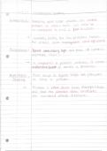
LECTURE I: Experimental Design terms; t-procedures (CI estimation and
testing)
t-Procedures
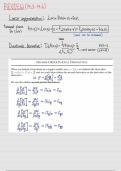
Goal: Analyze means using confidence intervals and hypothesis tests
Situations:
Situation 1: One sample, interest in population mean (assumes Normal
distribution).
Situation 2: Paired data (e.g., before/after), interest in mean of
differences.
Situation 3: Two independent samples, interest in the difference between
two means.
Assumptions:
- Independence
- Normality
- and (for Situation 3) equal variances.
Model Checks:
Independence: Depends on proper randomization.
Normality: Assessed using QQ plots.
Equal Variances: Checked using sample SDs, visual plots, and Levene’s
Test.
o If P > 0.05: Assume equal variances (use var.equal = TRUE in R).
o If P < 0.05: Use Welch’s t-test (var.equal = FALSE).
1
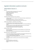
,LECTURE II: Sample size calculations & Wilcoxon tests.
1. Sample Size Calculations
Purpose: Determine the number of observations needed before collecting data,
based on how precise or powerful the study should be.
Two Main Research Aims:
Confidence Intervals: Define precision via:
o Desired width (or margin of error)
o Confidence level (typically 95%)
Hypothesis Testing: Define criteria via:
o Significance level α (e.g., 0.05) – type I error probability
o Minimum relevant difference ∆ (btw the true value & H0 value of
the parameter of interest)
o Power (probability of correctly rejecting H₀, typically ≥ 0.8) – type II
error probability
Key Idea: Required sample size depends on ∆, σ, α, and power.
Example: In a diet comparison, if ∆ = 3 is meaningful, and power = 0.8 is
desired, we can compute how many subjects are needed.
If power is too low (e.g., 0.25), the experiment may not be worth doing.
2. Wilcoxon Tests – For Non-Normal Data (Situations 1a, 2a, 3a)
When to Use: If Normality is questionable and sample size is small, t-
procedures may not be reliable Use non-parametric (rank-based) tests
instead.
Consequences of Non-Normality:
May shift focus from the mean to the median.
o Note in symmetric distributions: mode, median are the same – not in
non-symmetric distributions
t-tests become unreliable for small, skewed samples p-value no longer
reliable
Wilcoxon Tests:
Wilcoxon Rank Sum Test (Situation 3a: two independent samples)
o Shift alternative: the distributions of two population have to same
shape but may be shifted relative to each other
o Test statistic = sum of ranks for one group.
o Use R or PQRS output; understand expected value of rank sum
under H₀.
Wilcoxon Signed Rank Test (Situation 2a: paired samples)
o Assumes differences are symmetrically distributed around the
median.
o Test statistic = T+ or T− (sum of positive or negative ranks).
o Ignore Normal approximation or O&L’s method; rely on R/PQRS.
2
, Note on R Output: R uses a different form of test statistic (adjusted rank sum),
but you’re not required to compute it manually.
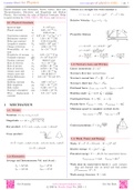
LECTURE III: Inference about one population proportion
Inference about the difference between two proportions or
probabilities
1. Inference for One Population Proportion (Situation 10)
Context: Binary outcomes (e.g. success/failure, diseased/healthy).
Key Parameter: π = true population proportion.
Sample Estimator:
𝜋̂ = y/n = observed proportion of successes.
y ~ Binomial(n, π).
Three Learning outcomes:
1. Confidence Interval for π
2. Binomial Test for a hypothesized π
3. Sample Size Calculation to achieve a desired confidence interval width
Binomial Test – Example Steps:
1. H₀: π = 0.3, Hₐ: π > 0.3
2. Test Statistic: y = number of "successes"
3. Distribution under H₀: y ~ Binomial(n = 20, π = 0.3)
4. One-tailed test → use Right P-value (RPV)
5. Reject H₀ if RPV ≤ 0.05
6. Sample result: y = 9
7. RPV = P(y ≥ 9) = 0.1134
8. Since 0.1134 > 0.05 → Fail to reject H₀
⚠ Note: Binomial is discrete, so LPV + RPV ≠ 1
⚠ Two-tailed P-value = 2 × min(LPV, RPV) but not always valid for skewed
distributions
2. Inference for the Difference Between Two Proportions (Situation 11)
Goal: Compare π₁ and π₂
Take two independent random samples:
o Group 1: n₁ individuals, y₁ "successes"
o Group 2: n₂ individuals, y₂ "successes"
Estimate π₁ − π₂ by: 𝜋̂₁ − 𝜋̂₂ = (y₁/n₁) − (y₂/n₂)
Tests for Difference Between Proportions:
We do NOT use z-tests.
We use Fisher’s Exact Test, based on the Hypergeometric
distribution (Vase model).
Vase Model (Hypergeometric Distribution):
N items total, K of type A (e.g. diseased), draw n items without
replacement.
3

