CFA Level 1 - 101 Must Knows Exam ||\\//|| ||\\//|| ||\\//|| ||\\//|| ||\\//|| ||\\//|| ||\\//|| ||\\//||
questions with verified detailed answers ||\\//|| ||\\//|| ||\\//|| ||\\//||
Addition Rule of Probability ||\\//|| ||\\//|| ||\\//||
ADDITION: P(A or B) = P(A) + P(B) - P(AB) ||\\//|| ||\\//|| ||\\//|| ||\\//|| ||\\//|| ||\\//|| ||\\//|| ||\\//|| ||\\//||
Roy's Safety First Criterion
||\\//|| ||\\//|| ||\\//||
Safety First Ratio = (E(R) - R)ₜ / σ
||\\//|| ||\\//|| ||\\//|| ||\\//|| ||\\//|| ||\\//|| ||\\//|| ||\\//||
Larger ratio is better ||\\//|| ||\\//|| ||\\//||
If (R)ₜ is risk free rate, then it becomes Sharpe Ratio
||\\//|| ||\\//|| ||\\//|| ||\\//|| ||\\//|| ||\\//|| ||\\//|| ||\\//|| ||\\//|| ||\\//||
Sharpe Ratio ||\\//||
Sharpe Ratio = (E(R) - RFR) / σ ||\\//|| ||\\//|| ||\\//|| ||\\//|| ||\\//|| ||\\//|| ||\\//||
Larger ratio is better ||\\//|| ||\\//|| ||\\//||
If (Rt) is higher than RFR, then it becomes Safety First Ratio
||\\//|| ||\\//|| ||\\//|| ||\\//|| ||\\//|| ||\\//|| ||\\//|| ||\\//|| ||\\//|| ||\\//|| ||\\//||
Central Limit Theorem ||\\//|| ||\\//||
,If we take samples of a population, with a large enough sample size, the distribution of all
||\\//|| ||\\//|| ||\\//|| ||\\//|| ||\\//|| ||\\//|| ||\\//|| ||\\//|| ||\\//|| ||\\//|| ||\\//|| ||\\//|| ||\\//|| ||\\//|| ||\\//|| ||\\//|| ||\\//||
sample means is normal with: ||\\//|| ||\\//|| ||\\//|| ||\\//||
- A mean equal to the population mean
||\\//|| ||\\//|| ||\\//|| ||\\//|| ||\\//|| ||\\//|| ||\\//||
- A variance equal to the population variance divided by sample size (σ² / n)
||\\//|| ||\\//|| ||\\//|| ||\\//|| ||\\//|| ||\\//|| ||\\//|| ||\\//|| ||\\//|| ||\\//|| ||\\//|| ||\\//|| ||\\//|| ||\\//||
Standard Error of Sample Mean ||\\//|| ||\\//|| ||\\//|| ||\\//||
σ / n^½ ||\\//|| ||\\//||
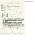
Binomial Probability ||\\//||
One of two possible outcomes (i.e. success/failure)
||\\//|| ||\\//|| ||\\//|| ||\\//|| ||\\//|| ||\\//||
Possible outcomes can be demonstrated in binomial tree ||\\//|| ||\\//|| ||\\//|| ||\\//|| ||\\//|| ||\\//|| ||\\//||
Use "nCr" on calculator to solve: ||\\//|| ||\\//|| ||\\//|| ||\\//|| ||\\//||
nCr = P(success)^x * P(failure)^(n-x) ||\\//|| ||\\//|| ||\\//|| ||\\//||
P - Value ||\\//|| ||\\//||
Based on a calculated test statistic, rather than a significance level (which is chosen)
||\\//|| ||\\//|| ||\\//|| ||\\//|| ||\\//|| ||\\//|| ||\\//|| ||\\//|| ||\\//|| ||\\//|| ||\\//|| ||\\//|| ||\\//||
p-value = smallest significance level at which an analyst can reject the null hypothesis ||\\//|| ||\\//|| ||\\//|| ||\\//|| ||\\//|| ||\\//|| ||\\//|| ||\\//|| ||\\//|| ||\\//|| ||\\//|| ||\\//|| ||\\//||
,one-tailed test - "less than or equal to" ||\\//|| ||\\//|| ||\\//|| ||\\//|| ||\\//|| ||\\//|| ||\\//||
two-tailed test - "equal to" ||\\//|| ||\\//|| ||\\//|| ||\\//||
Cumulative Distribution Function ||\\//|| ||\\//||
Gives the probability that a random variable will have an outcome less than or equal to a
||\\//|| ||\\//|| ||\\//|| ||\\//|| ||\\//|| ||\\//|| ||\\//|| ||\\//|| ||\\//|| ||\\//|| ||\\//|| ||\\//|| ||\\//|| ||\\//|| ||\\//|| ||\\//|| ||\\//||
specific value (represented by F(x)) ||\\//|| ||\\//|| ||\\//|| ||\\//||
F(x) = probability of an outcome less than or equal to x
||\\//|| ||\\//|| ||\\//|| ||\\//|| ||\\//|| ||\\//|| ||\\//|| ||\\//|| ||\\//|| ||\\//|| ||\\//||
Standard normal table (z) shows cumulative probabilities ||\\//|| ||\\//|| ||\\//|| ||\\//|| ||\\//|| ||\\//||
Effective Annual Yield ||\\//|| ||\\//||
EAY = (1 + (i/n))^n - 1
||\\//|| ||\\//|| ||\\//|| ||\\//|| ||\\//|| ||\\//||
Stated Rate = (EAY^(1/n) - 1) * n ||\\//|| ||\\//|| ||\\//|| ||\\//|| ||\\//|| ||\\//|| ||\\//||
Continuous Compounding ||\\//||
ln(EAY) = continuously compounded stated rate ||\\//|| ||\\//|| ||\\//|| ||\\//|| ||\\//||
e^(continuously compounded stated rate) = EAY ||\\//|| ||\\//|| ||\\//|| ||\\//|| ||\\//||
Type I Error ||\\//|| ||\\//||
Incorrectly rejecting a true null hypothesis ||\\//|| ||\\//|| ||\\//|| ||\\//|| ||\\//||
, (convicting an innocent person is Type I) ||\\//|| ||\\//|| ||\\//|| ||\\//|| ||\\//|| ||\\//||
Type II Error ||\\//|| ||\\//||
Failure to reject a false null hypothesis ||\\//|| ||\\//|| ||\\//|| ||\\//|| ||\\//|| ||\\//||
(failure to convict a guilty person is Type II) ||\\//|| ||\\//|| ||\\//|| ||\\//|| ||\\//|| ||\\//|| ||\\//|| ||\\//||
Significance Level / Power of a Test ||\\//|| ||\\//|| ||\\//|| ||\\//|| ||\\//|| ||\\//||
Significance Level = Probability of Type I ||\\//|| ||\\//|| ||\\//|| ||\\//|| ||\\//|| ||\\//||
Power of a Test = (1 - Probability of Type I) ||\\//|| ||\\//|| ||\\//|| ||\\//|| ||\\//|| ||\\//|| ||\\//|| ||\\//|| ||\\//|| ||\\//||
Covariance (Probability Model) ||\\//|| ||\\//||
Covariance of random variables A and B from probability model ||\\//|| ||\\//|| ||\\//|| ||\\//|| ||\\//|| ||\\//|| ||\\//|| ||\\//|| ||\\//||
On the calculator:
||\\//|| ||\\//||
1) Enter returns for set A and joint probabilities for AB; find mean A
||\\//|| ||\\//|| ||\\//|| ||\\//|| ||\\//|| ||\\//|| ||\\//|| ||\\//|| ||\\//|| ||\\//|| ||\\//|| ||\\//|| ||\\//||
2) Enter returns for set B and joint probabilities for AB; find mean B
||\\//|| ||\\//|| ||\\//|| ||\\//|| ||\\//|| ||\\//|| ||\\//|| ||\\//|| ||\\//|| ||\\//|| ||\\//|| ||\\//|| ||\\//||
3) Multiply each joint probability AB by each set's returns minus means
||\\//|| ||\\//|| ||\\//|| ||\\//|| ||\\//|| ||\\//|| ||\\//|| ||\\//|| ||\\//|| ||\\//|| ||\\//||
(ex: P(AB1)(A1 - Mean A)(B1 - Mean B) + P(AB2)(A2 - Mean A)(B2 - Mean B) + ... +
||\\//|| ||\\//|| ||\\//|| ||\\//|| ||\\//|| ||\\//|| ||\\//|| ||\\//|| ||\\//|| ||\\//|| ||\\//|| ||\\//|| ||\\//|| ||\\//|| ||\\//|| ||\\//|| ||\\//|| ||\\//|| ||\\//||
P(ABn)(An - Mean A)(Bn - Mean B)) ||\\//|| ||\\//|| ||\\//|| ||\\//|| ||\\//|| ||\\//||
4) The summed total is your covariance
||\\//|| ||\\//|| ||\\//|| ||\\//|| ||\\//|| ||\\//||
questions with verified detailed answers ||\\//|| ||\\//|| ||\\//|| ||\\//||
Addition Rule of Probability ||\\//|| ||\\//|| ||\\//||
ADDITION: P(A or B) = P(A) + P(B) - P(AB) ||\\//|| ||\\//|| ||\\//|| ||\\//|| ||\\//|| ||\\//|| ||\\//|| ||\\//|| ||\\//||
Roy's Safety First Criterion
||\\//|| ||\\//|| ||\\//||
Safety First Ratio = (E(R) - R)ₜ / σ
||\\//|| ||\\//|| ||\\//|| ||\\//|| ||\\//|| ||\\//|| ||\\//|| ||\\//||
Larger ratio is better ||\\//|| ||\\//|| ||\\//||
If (R)ₜ is risk free rate, then it becomes Sharpe Ratio
||\\//|| ||\\//|| ||\\//|| ||\\//|| ||\\//|| ||\\//|| ||\\//|| ||\\//|| ||\\//|| ||\\//||
Sharpe Ratio ||\\//||
Sharpe Ratio = (E(R) - RFR) / σ ||\\//|| ||\\//|| ||\\//|| ||\\//|| ||\\//|| ||\\//|| ||\\//||
Larger ratio is better ||\\//|| ||\\//|| ||\\//||
If (Rt) is higher than RFR, then it becomes Safety First Ratio
||\\//|| ||\\//|| ||\\//|| ||\\//|| ||\\//|| ||\\//|| ||\\//|| ||\\//|| ||\\//|| ||\\//|| ||\\//||
Central Limit Theorem ||\\//|| ||\\//||
,If we take samples of a population, with a large enough sample size, the distribution of all
||\\//|| ||\\//|| ||\\//|| ||\\//|| ||\\//|| ||\\//|| ||\\//|| ||\\//|| ||\\//|| ||\\//|| ||\\//|| ||\\//|| ||\\//|| ||\\//|| ||\\//|| ||\\//|| ||\\//||
sample means is normal with: ||\\//|| ||\\//|| ||\\//|| ||\\//||
- A mean equal to the population mean
||\\//|| ||\\//|| ||\\//|| ||\\//|| ||\\//|| ||\\//|| ||\\//||
- A variance equal to the population variance divided by sample size (σ² / n)
||\\//|| ||\\//|| ||\\//|| ||\\//|| ||\\//|| ||\\//|| ||\\//|| ||\\//|| ||\\//|| ||\\//|| ||\\//|| ||\\//|| ||\\//|| ||\\//||
Standard Error of Sample Mean ||\\//|| ||\\//|| ||\\//|| ||\\//||
σ / n^½ ||\\//|| ||\\//||
Binomial Probability ||\\//||
One of two possible outcomes (i.e. success/failure)
||\\//|| ||\\//|| ||\\//|| ||\\//|| ||\\//|| ||\\//||
Possible outcomes can be demonstrated in binomial tree ||\\//|| ||\\//|| ||\\//|| ||\\//|| ||\\//|| ||\\//|| ||\\//||
Use "nCr" on calculator to solve: ||\\//|| ||\\//|| ||\\//|| ||\\//|| ||\\//||
nCr = P(success)^x * P(failure)^(n-x) ||\\//|| ||\\//|| ||\\//|| ||\\//||
P - Value ||\\//|| ||\\//||
Based on a calculated test statistic, rather than a significance level (which is chosen)
||\\//|| ||\\//|| ||\\//|| ||\\//|| ||\\//|| ||\\//|| ||\\//|| ||\\//|| ||\\//|| ||\\//|| ||\\//|| ||\\//|| ||\\//||
p-value = smallest significance level at which an analyst can reject the null hypothesis ||\\//|| ||\\//|| ||\\//|| ||\\//|| ||\\//|| ||\\//|| ||\\//|| ||\\//|| ||\\//|| ||\\//|| ||\\//|| ||\\//|| ||\\//||
,one-tailed test - "less than or equal to" ||\\//|| ||\\//|| ||\\//|| ||\\//|| ||\\//|| ||\\//|| ||\\//||
two-tailed test - "equal to" ||\\//|| ||\\//|| ||\\//|| ||\\//||
Cumulative Distribution Function ||\\//|| ||\\//||
Gives the probability that a random variable will have an outcome less than or equal to a
||\\//|| ||\\//|| ||\\//|| ||\\//|| ||\\//|| ||\\//|| ||\\//|| ||\\//|| ||\\//|| ||\\//|| ||\\//|| ||\\//|| ||\\//|| ||\\//|| ||\\//|| ||\\//|| ||\\//||
specific value (represented by F(x)) ||\\//|| ||\\//|| ||\\//|| ||\\//||
F(x) = probability of an outcome less than or equal to x
||\\//|| ||\\//|| ||\\//|| ||\\//|| ||\\//|| ||\\//|| ||\\//|| ||\\//|| ||\\//|| ||\\//|| ||\\//||
Standard normal table (z) shows cumulative probabilities ||\\//|| ||\\//|| ||\\//|| ||\\//|| ||\\//|| ||\\//||
Effective Annual Yield ||\\//|| ||\\//||
EAY = (1 + (i/n))^n - 1
||\\//|| ||\\//|| ||\\//|| ||\\//|| ||\\//|| ||\\//||
Stated Rate = (EAY^(1/n) - 1) * n ||\\//|| ||\\//|| ||\\//|| ||\\//|| ||\\//|| ||\\//|| ||\\//||
Continuous Compounding ||\\//||
ln(EAY) = continuously compounded stated rate ||\\//|| ||\\//|| ||\\//|| ||\\//|| ||\\//||
e^(continuously compounded stated rate) = EAY ||\\//|| ||\\//|| ||\\//|| ||\\//|| ||\\//||
Type I Error ||\\//|| ||\\//||
Incorrectly rejecting a true null hypothesis ||\\//|| ||\\//|| ||\\//|| ||\\//|| ||\\//||
, (convicting an innocent person is Type I) ||\\//|| ||\\//|| ||\\//|| ||\\//|| ||\\//|| ||\\//||
Type II Error ||\\//|| ||\\//||
Failure to reject a false null hypothesis ||\\//|| ||\\//|| ||\\//|| ||\\//|| ||\\//|| ||\\//||
(failure to convict a guilty person is Type II) ||\\//|| ||\\//|| ||\\//|| ||\\//|| ||\\//|| ||\\//|| ||\\//|| ||\\//||
Significance Level / Power of a Test ||\\//|| ||\\//|| ||\\//|| ||\\//|| ||\\//|| ||\\//||
Significance Level = Probability of Type I ||\\//|| ||\\//|| ||\\//|| ||\\//|| ||\\//|| ||\\//||
Power of a Test = (1 - Probability of Type I) ||\\//|| ||\\//|| ||\\//|| ||\\//|| ||\\//|| ||\\//|| ||\\//|| ||\\//|| ||\\//|| ||\\//||
Covariance (Probability Model) ||\\//|| ||\\//||
Covariance of random variables A and B from probability model ||\\//|| ||\\//|| ||\\//|| ||\\//|| ||\\//|| ||\\//|| ||\\//|| ||\\//|| ||\\//||
On the calculator:
||\\//|| ||\\//||
1) Enter returns for set A and joint probabilities for AB; find mean A
||\\//|| ||\\//|| ||\\//|| ||\\//|| ||\\//|| ||\\//|| ||\\//|| ||\\//|| ||\\//|| ||\\//|| ||\\//|| ||\\//|| ||\\//||
2) Enter returns for set B and joint probabilities for AB; find mean B
||\\//|| ||\\//|| ||\\//|| ||\\//|| ||\\//|| ||\\//|| ||\\//|| ||\\//|| ||\\//|| ||\\//|| ||\\//|| ||\\//|| ||\\//||
3) Multiply each joint probability AB by each set's returns minus means
||\\//|| ||\\//|| ||\\//|| ||\\//|| ||\\//|| ||\\//|| ||\\//|| ||\\//|| ||\\//|| ||\\//|| ||\\//||
(ex: P(AB1)(A1 - Mean A)(B1 - Mean B) + P(AB2)(A2 - Mean A)(B2 - Mean B) + ... +
||\\//|| ||\\//|| ||\\//|| ||\\//|| ||\\//|| ||\\//|| ||\\//|| ||\\//|| ||\\//|| ||\\//|| ||\\//|| ||\\//|| ||\\//|| ||\\//|| ||\\//|| ||\\//|| ||\\//|| ||\\//|| ||\\//||
P(ABn)(An - Mean A)(Bn - Mean B)) ||\\//|| ||\\//|| ||\\//|| ||\\//|| ||\\//|| ||\\//||
4) The summed total is your covariance
||\\//|| ||\\//|| ||\\//|| ||\\//|| ||\\//|| ||\\//||