Summary Business Research Methods - prof Cleeren

BRM – Cleeren



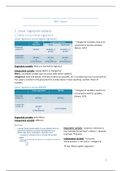
1. Linear regression analysis
1.1 When to use a linear regression?
Linear regression versus logistic regression?
* Categorical variables need to be
converted to dummy variables
(binary: 1/0)!




Dependent variable: Metric or nominal (in logistics)

Independent variable: always Metric or Categorical
Metric: countable variable (you can count with these numbers).
Categorical: male and female, all kinds of values are possible, isn’t a number (you can’t count with it).
You assign a number to the group but the number doesn’t mean anything, random choice of
numbers.

Linear regression versus ANOVA?
* Categorical variables need to be
converted to dummy variables
(binary: 1/0)!




Dependent variable: both Metric
Independent variable: different

Exercise
Dependent variable: “a person´s decision to
buy a private (store) label” ≠ Metric = Nominal
(2 groups → binary)

Independent variable: “consumer
characteristics” ≠ not metric = categorical

→ Test: Binary logistic regression




1

, Dependent variable: “a person´s attitude
towards buying private (store) label” = Likert
scale → considered a Metric variable.

Independent variable: “consumer
characteristics” ≠ not metric = categorical

→ Test: Linear regression

Dependent variable: “a person´s attitude
towards buying private (store) label” =
Nominal (>2 groups)

Independent variable: “consumer
characteristics” ≠ not metric = categorical

→ Multinomial logistic regression


1.2 Creating dummy variables
• Transform categorical independent variables into dummy (1/0) variables (aka indicator
variables) in a linear (and logistic) regression
• Dummy variable trap!
o = if you would include as many dummies as response categories → you create perfect
multicollinearity, you can perfectly predict values of last category based on values of
other categories. If male = 1 → female will be 0.
o # dummies = # response categories – 1
▪ You should include 1 dummy less than the number of response categories.

HOW: Tabulate X, generate(X)

Example linear regression




2

, Control variable = which we know will influence
dependent variable/results, but we are not really
interested in their effect (there will not be a
hypothesis on this). If we do not include them →
omitted variable bias. They will be treated as
independent variables.

Subscript (i) = level of observation !


1.3 Linear regression in Stata
HOW: Regress

1.3.1 Model diagnostics – Steps
• Step 1: Check assumptions (if necessary, apply corrections)
o Assumption 1: Causality.
o Assumption 2: Were all relevant variables included?
o Assumption 3: Metric dependent variable.
o Assumption 4: Linear relationship between dependent and independent variables.
o Assumption 5: Additive relationship between dependent and independent variables.
o Assumption 6: Residuals need to be independent, normally distributed, homoscedastic,
without autocorrelation.
o Assumption 7: Enough observations
o Assumption 8: No multicollinearity
o Assumption 9: No extreme values
• Step 2: Check ‘meaningfulness’ of model (model fit); H0: R² = 0
• Step 3: Interpret the coefficients of each independent variable; H0: bi = 0

Step 1: check assumptions
ASSUMPTION 1: CAUSALITY
• Independent variables (RHS) should be causing the dependent variable.

ASSUMPTION 2: ALL RELEVANT VARIABLES
• No extreme clusters & No striking patterns
HOW: residuals versus fitted (rvf) plot - Predicted variables against residuals

ASSUMPTION 6: NORMAL DISTRIBUTION OF RESIDUALS
HOW visually: Histogram of residuals – should be normally distributed
PP-plot (probability-plot) – should be normally distributed

HOW statistically: Shapiro’s Wilk normality test – H0: residuals normally distributed
! You don’t want to reject H0, residuals will then be normally distributed.

• If violated: check why the standard errors are not normally distributed:
o Problem in model -> fix it!
o Dependent variable not normally distributed -> transformation of dependent variable
(logarithm, square, root)
• Important: if you use a transformation, it has implications for the interpretation of the results !!
(interpret in function of transformed variable).

• If the sample size is large enough → violation of normal distribution usually not a problem


3