WEEK 3b
. Introduction
2
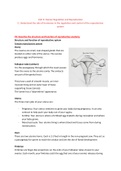
. Discrete bivariate distributions
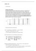
Joint / simultaneous probabilities -> centre of table
– e.g. P(1,2) = P(X=1 and Y=2) = 0.09
– In this example 12 possible joint outcomes (3x4)
A joint distribution has the following requirements:
Marginal probability distribution -> last row for X / last column for Y
– Of X the value of Y doesn’t play a role
– It is a population distribution of one random variable -> can be used to
1 calculate the population mean and variance of X or Y
, Conditional probability distributions - e.g.:
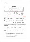
The three conditional probabilities sum up to 1, as it is a complete
distribution
Conditional expectation = the expected value of X, when the value of Y is
already known
e.g.
Formula:
Conditional variance = variance of X, when Y is known
Formula:
. Introduction
2
. Discrete bivariate distributions
Joint / simultaneous probabilities -> centre of table
– e.g. P(1,2) = P(X=1 and Y=2) = 0.09
– In this example 12 possible joint outcomes (3x4)
A joint distribution has the following requirements:
Marginal probability distribution -> last row for X / last column for Y
– Of X the value of Y doesn’t play a role
– It is a population distribution of one random variable -> can be used to
1 calculate the population mean and variance of X or Y
, Conditional probability distributions - e.g.:
The three conditional probabilities sum up to 1, as it is a complete
distribution
Conditional expectation = the expected value of X, when the value of Y is
already known
e.g.
Formula:
Conditional variance = variance of X, when Y is known
Formula: