Experimental Research Methods
Lecture 1
Descriptive statistics
• Descriptive statistics = summarize data
• Data = numerical information of a population or sample
Population→All members of a defined group, Parameters are measures of properties of scores in the population,
Parameters are denoted with Greek letters (μ, σ)
Sample→ Subset of members of a defined group, Sample statistics are measures of properties of the scores in the
sample, Sample statistics are denoted with Latin letters (X, s)
Descriptive statistics
• Data from a sample: 1 1 4 4 3 2 3 1 2 1 3 4 4 3 3 4 4 3 1 4 4 4 4 3 4 4 2 3 1 3 4 1 3 4 4 4 2 4 2 4 3 3 1 1 4 3 4 1 3
• Descriptive statistics help summarize the data → list of raw data is unclear
• Two ways to summarize data: 1. With a distribution 2. With sample statistics
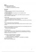
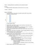
Distribution
• Data summarized by grouping data with the same score
• This can be done by using a frequency distribution or histogram
• SPSS syntax to generate frequency distribution and histogram: (syntax is important in this course!):
FREQUENCIES VARIABLES=x /HISTOGRAM /ORDER= ANALYSIS .
Sample statistics
- Data summarized using characteristic features of the distribution
- What are the characteristic features of a distribution?
1. Most characteristic score of a distribution=central tendency
2. How much do scores deviate from the most characteristic score=dispersion
Central tendency: mean, median and mode→mean is the sum of all scores divided by the total number of scores
Dispersion: range, variance and standard deviation
Variance is the sum of all squared deviation scores divided by the number of scores divided by the number of scores
minus one. Standard deviation is the square root of the variance (s)
Inferential statistics
• Descriptive statistics suffices if we have data of the entire population
• However, almost always we only have data of a sample and not the population, because:
1. Too expensive 2. It takes too long to collect these data 3. Sometimes impossible
• Using inferential statistics, we can draw conclusions about a population based on a sample
• There are three “procedures” in inferential statistics:
1. Hypothesis testing 2. Point estimation 3. Interval estimation→ confidence intervals
Hypothesis testing
• Question: What is the mean of the population from which a sample of 50 cases was drawn?
• In hypothesis testing, you examine whether the mean of the population is equal to a certain value or not → hypotheses
are exclusive and exhaustive • Example: H0: μ = 2.5 and H1: μ ≠ 2.5
• Here, we discuss a two-sided test (H1 contains ≠), later we discuss a one-sided test (H1 contains > of <)
• You test whether you can reject H0 or not. If you reject H0, you conclude H1, i.e. is not equal to 2.5
• Rules of thumb for creating hypotheses:
1. H0 contains “=“ →always the case
2. H1 contains expectations of researcher → often, but not always the case
Steps in hypothesis testing
Step 1: Formulate hypotheses H0: μ = 2.5 and H1: μ ≠ 2.5
Step 2: Determine decision rule to decide when a result is statistically significant p ≤ α
Step 3: Determine p-value based on SPSS output
Step 4: Decision on significance and conclusion
Apply to our example: Syntax
T-TEST /TESTVAL=2.5 /MISSING=ANALYSIS /VARIABLES=x /CRITERIA=CIN (.95) .
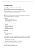
Logic hypothesis testing
1
,- You make an assumption about the value of a parameter (here μ) the null hypothesis (step 1)
- Assuming that this value is true, you determine the possible values the sample statistic (here X_) can take (sampling
distribution of X_) in a simple random sample of N cases
- The mean of the sample distribution is μ, the variance is σ²/N
- Using that sampling distribution, you determine the probability, p-value, that value of X_ or a more extreme value occurs
- In Step 3 you determine the position of X_ in the sampling distribution, do you also implicitly determine the p-value
- If the p value is lower than a you conclude→ If my H0 is true, then the probability that I observe this value for X_ or an
even more extreme value is quite smaller than a. This probability is so small that I do not trust my null hypothesis
anymore. I reject H0
- If the p value is larger than a you conclude→If my H0 is true, then the probability that I observe this value for X_ or an
even more extreme value is quite large. I don’t have enough reasons to doubt the correctness of H0. I do not reject H0
Remark:
One of the assumptions is that the sample is a ‘simple random sample’, meaning:
- All cases have an equal chance to be sampled
- Cases are selected independently of one another
The test cannot be used if these assumptions are not met
One-sided vs. two-sided testing
• Logic for one-sided and two-sided testing is the same
• However, SPSS output is always two-sided, so...
• convert two-sided “Sig.” in SPSS output to the correct (one-sided) p-value
• We can use the super slide on the next slide for this
Manual interpretation ‘Sig.’ in SPSS output
• In all cases below, the following decision rule holds:
Point estimation
- Point estimation is used to answer the following question: What is the best guess of this parameter?
- So… which values lies closest to the population value
In the case of the mean, the best guess is X_ In the case of the variance, the best guess is s²
Interval estimation
- With confidence intervals, you answer the following question: What is the interval in which the value of the parameter
lies …% confidence?
- A 95% confidence interval for μ: In 95% of the times I draw a sample of N=50, the confidence interval will contain μ
- Formula confidence interval:
Relation confidence intervals and testing
- You can use confidence intervals to test two-sided hypothesis:
- Decision rule: Two-sided test with significance level a
Why does this decision rule work?
Assume H0 is true (=starting point hypothesis test)
- 95% of all possible samples will produce a CI95 in which μH0 falls (correctly not rejecting H0)
- 5% of all possible samples will produce a CI95 in which μH0 does not fall (incorrectly rejecting H0=Type I error)
2
,Alternative interpretation CI in relation with hypothesis testing
→The CI fives all possible hypothetical values for μ that are not rejected by the sample statistics (given a)
Testing means
3-5 >>
Example test two independent samples
• Example from “Survival Manual” from Pallant (Chapter 17)
• Research question: On average, do male and female students differ in their self-esteem?
Step 1: Formulate hypotheses: H0: F = M and H1: F ≠ M
Step 2: When is a result significant? p < a = 0.05
Step 3: Determine p-value based on SPSS output
• Always interpret Levene’s test in contrast to Warner’s recommendation (book I, p. 333)
Step 4: Decision on significance and conclusion:
p = 0,105 > 0,05, so H0 cannot be rejected: “Average self-esteem does not differ between male and female students”
Lecture 2
Power of a test
• If we test, we want to draw the correct conclusion:
• If H0 is true, do not reject H0 • If H1 is true, reject H0
• What is the probability for drawing the correct conclusion?
• Say a researcher expects that having fewer police officers on the street will decrease safety
Type I→false positive conclusion
Type II error→there is an effect in reality, but we don’t find the effect in the test
alpha=significance threshold →5% chance in every test of drawing a false positive (type I error) →less probability of type I
error when alpha is lower
betha→probability of not detecting a true effect →hard not to detect betha because it relates to the power of the effect
• The power of a test is the probability of correctly rejecting the null hypothesis if this is indeed the correct decision
how likely it is that you will find a true effect
• Therefore, a highly powered test is preferred, as it implies a better probability to correctly reject the null hypothesis
Determining power of a z-test
Sample size→the more you look the more likely to find it→bigger sample size>>
It is easier to find a big object than a small one→bigger effects easier to find
How messy it is→if really messy, more difficult to find the effect (standard deviation)
3
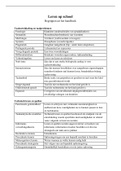
, Steps for determining power:
You need a specific alternative hypothesis (i.e. hypothesize an exact value)
1. Determine the critical Zcv for the given H0 (and the assumed alpha and direction of a test) critical value=1.96 for a=.05
2. Convert this Zcv to the corresponding x-value, x_cv (number scale of the value, eg. cm)
3. Convert the critical value x_cv to the Zh1 value for the given H1 (look at the critical value, ends of the curve)
if we want to test for power we have to choose a point alternative hypothesis (a specific value, usually it was H0 mean=2,
H1 different than 2, here H1 mean=4 →value for which we reject H0→we can calculate power only if we pick a specific
value for the alternative hypothesis)
4. The power is equal to the probability: P(Z ≥ ZH1 I H1) given that the H1 is true
eg. Ho mean>= 64.6, H1 mean=60.7
calculate standard error (calculate means in infinite number of samples→hypothetical standard deviation of the mean
error is the standard error→allows us to do probability calculus about hypotheses)
(standard deviation=8.9 sample=91) =9.3 (width of the curve)
LINK SLIDE 5 → tool to practice + draw situations yourself
lower alpha→lower power→you will miss more true effects, but will be less likely to make type 1 errors→betha increases
z-test look at critical value table, t-test look at the t-value test
Power of a test
• Back to the start: we want to have the largest probability of making correct decisions
• small alpha • Power (1-betha) large
• We determine alpha ourselves (criterion for deciding we find something), how do we influence power?
• Four factors that influence power:
• ∝ (when we conclude “we found something”)
• N (how “long” we’re looking: if you check 10.000 participants, you’re more likely to find something than if you check 10
• σ (how “noisy” the data are; more noise makes it harder to find an effect) bif standard deviation=noisy data
• The ‘true μ’ in the alternative hypothesis (H1) (bigger effects are easier to find)
• Practice with calculating power in the first tutorial
• Note: Often one question about calculating power on the exam
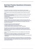
Effect size
• When H0 is rejected based on a hypothesis test, scientific claims get the label ‘significant’ (... hurray!) But often they
publish false positive conclusions→alpha=5% → 20 students get back one significant result for sure→write the study and
publish because found a significant effect→but could be a false positive→do not pass replication 73% of psychological
findings did not reproduce/replicate→having high power and looking for large effect sizes can fix this
• But ‘significant’ does not mean that is has definitively been proven that there is a systematic effect (contrary to what
some people make you want to believe). Why not?
• And... significant does also not mean that the effect is practically/clinically relevant. Even very small – uninteresting –
differences can be significant if you use a very big sample. • ... because
• If N is small, power is small, statistically not significant, even if effect is large
• If N is big, power is large, statistically significant, even if effect is small
eg. standard error decreases as the sample size increases, then test statistic gets bigger (t-statistic) and p-value
decreases→so if you want a significant result get big sample size
- A measure of the effect size is desirable to determine if an effect is meaningful: How large is the effect that we observe
in our sample?
- “ For readers to appreciate the magnitude or importance of a study’s findings, it is recommended to include some
measure of effect size in the Results section. The general principle to follow is to provide readers with enough information
to assess the magnitude of the observed effect”
- 2 important measures of the effect size when comparing means:
1. Cohen’s d →how large is the relative difference in the groups? Effect sizes between groups
2. (Partial) explained variance η² →how much of the variance is explained by group membership?
- Rule of thumb interpretative effect size: ( d , η² )
small (0.2, 0.01) medium (0.5, 0.06) Large (0.8, 0.14)
4
Lecture 1
Descriptive statistics
• Descriptive statistics = summarize data
• Data = numerical information of a population or sample
Population→All members of a defined group, Parameters are measures of properties of scores in the population,
Parameters are denoted with Greek letters (μ, σ)
Sample→ Subset of members of a defined group, Sample statistics are measures of properties of the scores in the
sample, Sample statistics are denoted with Latin letters (X, s)
Descriptive statistics
• Data from a sample: 1 1 4 4 3 2 3 1 2 1 3 4 4 3 3 4 4 3 1 4 4 4 4 3 4 4 2 3 1 3 4 1 3 4 4 4 2 4 2 4 3 3 1 1 4 3 4 1 3
• Descriptive statistics help summarize the data → list of raw data is unclear
• Two ways to summarize data: 1. With a distribution 2. With sample statistics
Distribution
• Data summarized by grouping data with the same score
• This can be done by using a frequency distribution or histogram
• SPSS syntax to generate frequency distribution and histogram: (syntax is important in this course!):
FREQUENCIES VARIABLES=x /HISTOGRAM /ORDER= ANALYSIS .
Sample statistics
- Data summarized using characteristic features of the distribution
- What are the characteristic features of a distribution?
1. Most characteristic score of a distribution=central tendency
2. How much do scores deviate from the most characteristic score=dispersion
Central tendency: mean, median and mode→mean is the sum of all scores divided by the total number of scores
Dispersion: range, variance and standard deviation
Variance is the sum of all squared deviation scores divided by the number of scores divided by the number of scores
minus one. Standard deviation is the square root of the variance (s)
Inferential statistics
• Descriptive statistics suffices if we have data of the entire population
• However, almost always we only have data of a sample and not the population, because:
1. Too expensive 2. It takes too long to collect these data 3. Sometimes impossible
• Using inferential statistics, we can draw conclusions about a population based on a sample
• There are three “procedures” in inferential statistics:
1. Hypothesis testing 2. Point estimation 3. Interval estimation→ confidence intervals
Hypothesis testing
• Question: What is the mean of the population from which a sample of 50 cases was drawn?
• In hypothesis testing, you examine whether the mean of the population is equal to a certain value or not → hypotheses
are exclusive and exhaustive • Example: H0: μ = 2.5 and H1: μ ≠ 2.5
• Here, we discuss a two-sided test (H1 contains ≠), later we discuss a one-sided test (H1 contains > of <)
• You test whether you can reject H0 or not. If you reject H0, you conclude H1, i.e. is not equal to 2.5
• Rules of thumb for creating hypotheses:
1. H0 contains “=“ →always the case
2. H1 contains expectations of researcher → often, but not always the case
Steps in hypothesis testing
Step 1: Formulate hypotheses H0: μ = 2.5 and H1: μ ≠ 2.5
Step 2: Determine decision rule to decide when a result is statistically significant p ≤ α
Step 3: Determine p-value based on SPSS output
Step 4: Decision on significance and conclusion
Apply to our example: Syntax
T-TEST /TESTVAL=2.5 /MISSING=ANALYSIS /VARIABLES=x /CRITERIA=CIN (.95) .
Logic hypothesis testing
1
,- You make an assumption about the value of a parameter (here μ) the null hypothesis (step 1)
- Assuming that this value is true, you determine the possible values the sample statistic (here X_) can take (sampling
distribution of X_) in a simple random sample of N cases
- The mean of the sample distribution is μ, the variance is σ²/N
- Using that sampling distribution, you determine the probability, p-value, that value of X_ or a more extreme value occurs
- In Step 3 you determine the position of X_ in the sampling distribution, do you also implicitly determine the p-value
- If the p value is lower than a you conclude→ If my H0 is true, then the probability that I observe this value for X_ or an
even more extreme value is quite smaller than a. This probability is so small that I do not trust my null hypothesis
anymore. I reject H0
- If the p value is larger than a you conclude→If my H0 is true, then the probability that I observe this value for X_ or an
even more extreme value is quite large. I don’t have enough reasons to doubt the correctness of H0. I do not reject H0
Remark:
One of the assumptions is that the sample is a ‘simple random sample’, meaning:
- All cases have an equal chance to be sampled
- Cases are selected independently of one another
The test cannot be used if these assumptions are not met
One-sided vs. two-sided testing
• Logic for one-sided and two-sided testing is the same
• However, SPSS output is always two-sided, so...
• convert two-sided “Sig.” in SPSS output to the correct (one-sided) p-value
• We can use the super slide on the next slide for this
Manual interpretation ‘Sig.’ in SPSS output
• In all cases below, the following decision rule holds:
Point estimation
- Point estimation is used to answer the following question: What is the best guess of this parameter?
- So… which values lies closest to the population value
In the case of the mean, the best guess is X_ In the case of the variance, the best guess is s²
Interval estimation
- With confidence intervals, you answer the following question: What is the interval in which the value of the parameter
lies …% confidence?
- A 95% confidence interval for μ: In 95% of the times I draw a sample of N=50, the confidence interval will contain μ
- Formula confidence interval:
Relation confidence intervals and testing
- You can use confidence intervals to test two-sided hypothesis:
- Decision rule: Two-sided test with significance level a
Why does this decision rule work?
Assume H0 is true (=starting point hypothesis test)
- 95% of all possible samples will produce a CI95 in which μH0 falls (correctly not rejecting H0)
- 5% of all possible samples will produce a CI95 in which μH0 does not fall (incorrectly rejecting H0=Type I error)
2
,Alternative interpretation CI in relation with hypothesis testing
→The CI fives all possible hypothetical values for μ that are not rejected by the sample statistics (given a)
Testing means
3-5 >>
Example test two independent samples
• Example from “Survival Manual” from Pallant (Chapter 17)
• Research question: On average, do male and female students differ in their self-esteem?
Step 1: Formulate hypotheses: H0: F = M and H1: F ≠ M
Step 2: When is a result significant? p < a = 0.05
Step 3: Determine p-value based on SPSS output
• Always interpret Levene’s test in contrast to Warner’s recommendation (book I, p. 333)
Step 4: Decision on significance and conclusion:
p = 0,105 > 0,05, so H0 cannot be rejected: “Average self-esteem does not differ between male and female students”
Lecture 2
Power of a test
• If we test, we want to draw the correct conclusion:
• If H0 is true, do not reject H0 • If H1 is true, reject H0
• What is the probability for drawing the correct conclusion?
• Say a researcher expects that having fewer police officers on the street will decrease safety
Type I→false positive conclusion
Type II error→there is an effect in reality, but we don’t find the effect in the test
alpha=significance threshold →5% chance in every test of drawing a false positive (type I error) →less probability of type I
error when alpha is lower
betha→probability of not detecting a true effect →hard not to detect betha because it relates to the power of the effect
• The power of a test is the probability of correctly rejecting the null hypothesis if this is indeed the correct decision
how likely it is that you will find a true effect
• Therefore, a highly powered test is preferred, as it implies a better probability to correctly reject the null hypothesis
Determining power of a z-test
Sample size→the more you look the more likely to find it→bigger sample size>>
It is easier to find a big object than a small one→bigger effects easier to find
How messy it is→if really messy, more difficult to find the effect (standard deviation)
3
, Steps for determining power:
You need a specific alternative hypothesis (i.e. hypothesize an exact value)
1. Determine the critical Zcv for the given H0 (and the assumed alpha and direction of a test) critical value=1.96 for a=.05
2. Convert this Zcv to the corresponding x-value, x_cv (number scale of the value, eg. cm)
3. Convert the critical value x_cv to the Zh1 value for the given H1 (look at the critical value, ends of the curve)
if we want to test for power we have to choose a point alternative hypothesis (a specific value, usually it was H0 mean=2,
H1 different than 2, here H1 mean=4 →value for which we reject H0→we can calculate power only if we pick a specific
value for the alternative hypothesis)
4. The power is equal to the probability: P(Z ≥ ZH1 I H1) given that the H1 is true
eg. Ho mean>= 64.6, H1 mean=60.7
calculate standard error (calculate means in infinite number of samples→hypothetical standard deviation of the mean
error is the standard error→allows us to do probability calculus about hypotheses)
(standard deviation=8.9 sample=91) =9.3 (width of the curve)
LINK SLIDE 5 → tool to practice + draw situations yourself
lower alpha→lower power→you will miss more true effects, but will be less likely to make type 1 errors→betha increases
z-test look at critical value table, t-test look at the t-value test
Power of a test
• Back to the start: we want to have the largest probability of making correct decisions
• small alpha • Power (1-betha) large
• We determine alpha ourselves (criterion for deciding we find something), how do we influence power?
• Four factors that influence power:
• ∝ (when we conclude “we found something”)
• N (how “long” we’re looking: if you check 10.000 participants, you’re more likely to find something than if you check 10
• σ (how “noisy” the data are; more noise makes it harder to find an effect) bif standard deviation=noisy data
• The ‘true μ’ in the alternative hypothesis (H1) (bigger effects are easier to find)
• Practice with calculating power in the first tutorial
• Note: Often one question about calculating power on the exam
Effect size
• When H0 is rejected based on a hypothesis test, scientific claims get the label ‘significant’ (... hurray!) But often they
publish false positive conclusions→alpha=5% → 20 students get back one significant result for sure→write the study and
publish because found a significant effect→but could be a false positive→do not pass replication 73% of psychological
findings did not reproduce/replicate→having high power and looking for large effect sizes can fix this
• But ‘significant’ does not mean that is has definitively been proven that there is a systematic effect (contrary to what
some people make you want to believe). Why not?
• And... significant does also not mean that the effect is practically/clinically relevant. Even very small – uninteresting –
differences can be significant if you use a very big sample. • ... because
• If N is small, power is small, statistically not significant, even if effect is large
• If N is big, power is large, statistically significant, even if effect is small
eg. standard error decreases as the sample size increases, then test statistic gets bigger (t-statistic) and p-value
decreases→so if you want a significant result get big sample size
- A measure of the effect size is desirable to determine if an effect is meaningful: How large is the effect that we observe
in our sample?
- “ For readers to appreciate the magnitude or importance of a study’s findings, it is recommended to include some
measure of effect size in the Results section. The general principle to follow is to provide readers with enough information
to assess the magnitude of the observed effect”
- 2 important measures of the effect size when comparing means:
1. Cohen’s d →how large is the relative difference in the groups? Effect sizes between groups
2. (Partial) explained variance η² →how much of the variance is explained by group membership?
- Rule of thumb interpretative effect size: ( d , η² )
small (0.2, 0.01) medium (0.5, 0.06) Large (0.8, 0.14)
4