The Top-Hat function
JT(x)dx
T() =
9) =
1 The area of the top-hat function is 1
·
Height Tak) =
aT(x) area =
a
·
Width Tb(x) =
T(b) bc1 : narrower bc1 : wider area = 'b
·
Translation Tc(x-c) O :
righ co : left centredate area = 1
Tabc(x) =
aT() height =
a width = b centred atc area = ab
The Gaussian Function
G() = e [Gbd =I x = n =
1
Height Gal) =
aG(x) area a
·
=
·
Width Gp(x) G(xb) =
bc1 : narrower bc1 : wider area = 'b
·
Translation Gc(x c -
O :
righ co : left centredate area = 1
Gapc(x) =
a e-P" centredate area = ab
Th
The Lorentzian
((x) = i It shorter and fatter than a Gaussian
& ((x)dx =
= ((dx =
En =
1
I
Gapc(x) centredatc area= a
& p
l
= a
+
The Dirac Delta function
We can construct Tabc() Gabc (2) and Labe (2) to have unit area 1 by choosing a =.
, ,
Assuming the functions are centred at 0 (c 0) we get a one-parameter family of functions =
.
1
Tob = T() Go() + G()=
= -E (y(x) = ((z) =
bit1 +
1-
We can consider the limit be of : the functions become infinitely tall and narrow ,
still with area = 1
D
f(x) =
limG( =
lim J(x) =
lim() Li+ =
ba +x
b-o be
,The function is zero everywhere but the origin .
It has an integral of I
Uses of J(C) : ·
in classical mechanics and electromagnetism it represents the mass density or charge density of a
particle that is perfectly localised at the origin . The mass is given by the integral for a particle ,
with mass #1 simply multiply the delta function by the mass.
,
·
In quantum mechanics it represents the probability density of a
particle that has a definite
position . This is
automatically normalised as the delta function has area I
Since PG) = /TbdK and PCC) =(2) then MDC = OG)
·
( g(x)(dx =
g(d)(- ((x)dx =
g(0)
· (oh()G( -
a)dx = h(a)( - 0x -
a)dx =
h(a)
· J% Off() d = where c is a root of f(x)
(%
1
·
G(as)dx = G(ax) =
ad()
·
106 = 1 (50 = 0 (o(x + 2) =
1 Take care with finite intervals
M
The delta function has
(SG) de =
dimensionless units that
·
G() has units m are the inverse of its argument
.
The Kronecker Delta
dij Eberwise CiGij
= = C; The Kronecker delta picks out a term from a um a
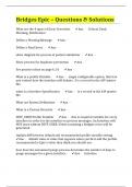
Fourier Series
for a function on an interval
eg .
a
guitar string from
= 0 to (C = (
The guitar string obeys a linear wave equation
Oy
:
The solutions of this equation are
standing waves yn (x .
t) =
An Sin (Kn > ) cos (Wnt + On)
where the wave number of the nth mode and the vkn
is : kn = not
angular frequency : Wn = =
nev
I L
Because the wave equation is linear any sum of solutions is also a solution .
,
Any function y (x) that satisfies the same boundary conditions can be written as a suitably weighted sum
of the functions yn (x).
, We can write (2) as a sum of the basis functions Yn() and then add in the time evolution :
y
y
( %) , = Usin (knx) =
y(x t),
= ansin (knx)cos(wnt)
We can determine the coefficients an by exploiting the fact that the basis functions sin (knx) sin
(n)
=
form an orthonormal set :
Elo yn() ym()dx =
Em Soherwise
Hence we can isolate a particular fourier coefficient by "dotting in" the corresponding basis function from the
left :
if y(x) = any
then"ymybdx = any(y(dx = =
/
Hence : am =
ym()yc where
ym() = sin
(mix)
Fourier Transform
Similar to fourier series but on an infinite interval.
for kn =
At as -o the kn values become closer
together they tend to
-
a continuum
L
We canfunction i (K) the Fourier Transform of the real-space function y
define a ,
() which tells
,
us how much of
fourier harmonic k is required to construct the real space function (x)
y .
The real-space function y (x) is defined on the whole real line whilst the fourier transform (k) is defined only on the
,
half-line ke(0 0) because y (2) is real We can extend our considerations to complex functions to complete the
,
.
symmetry.
Fourier's theorem tells us that
any complex function y () on the real line can be written as a
weighted sum of plane
waves :
-
ilD
(x) e where I take
any real value from o to [K is continuous
integrate
y, can so now we can
= o
-
.
y(x) = (e "(y(kdk ·
when k q the complex exponentials cancel
=
and the
integrand is 1 /% dx is infinite
(e ge id
:
:
Orthonormality : consider the overlap integral ·
whenk & the plane waves oscillate out of
phase with equal amounts of constructive and
This presents the Dirac delta function (il- =
25(q-k) destructive interference thus,giving zero
To calculate the fourier transform we use the orthonormality relation :
↑ eyedx =
((k)dk. e-idx =
(8y(10(17-9)dk
y(q)
j(k) Je
=
:
=
y(x)dx
JT(x)dx
T() =
9) =
1 The area of the top-hat function is 1
·
Height Tak) =
aT(x) area =
a
·
Width Tb(x) =
T(b) bc1 : narrower bc1 : wider area = 'b
·
Translation Tc(x-c) O :
righ co : left centredate area = 1
Tabc(x) =
aT() height =
a width = b centred atc area = ab
The Gaussian Function
G() = e [Gbd =I x = n =
1
Height Gal) =
aG(x) area a
·
=
·
Width Gp(x) G(xb) =
bc1 : narrower bc1 : wider area = 'b
·
Translation Gc(x c -
O :
righ co : left centredate area = 1
Gapc(x) =
a e-P" centredate area = ab
Th
The Lorentzian
((x) = i It shorter and fatter than a Gaussian
& ((x)dx =
= ((dx =
En =
1
I
Gapc(x) centredatc area= a
& p
l
= a
+
The Dirac Delta function
We can construct Tabc() Gabc (2) and Labe (2) to have unit area 1 by choosing a =.
, ,
Assuming the functions are centred at 0 (c 0) we get a one-parameter family of functions =
.
1
Tob = T() Go() + G()=
= -E (y(x) = ((z) =
bit1 +
1-
We can consider the limit be of : the functions become infinitely tall and narrow ,
still with area = 1
D
f(x) =
limG( =
lim J(x) =
lim() Li+ =
ba +x
b-o be
,The function is zero everywhere but the origin .
It has an integral of I
Uses of J(C) : ·
in classical mechanics and electromagnetism it represents the mass density or charge density of a
particle that is perfectly localised at the origin . The mass is given by the integral for a particle ,
with mass #1 simply multiply the delta function by the mass.
,
·
In quantum mechanics it represents the probability density of a
particle that has a definite
position . This is
automatically normalised as the delta function has area I
Since PG) = /TbdK and PCC) =(2) then MDC = OG)
·
( g(x)(dx =
g(d)(- ((x)dx =
g(0)
· (oh()G( -
a)dx = h(a)( - 0x -
a)dx =
h(a)
· J% Off() d = where c is a root of f(x)
(%
1
·
G(as)dx = G(ax) =
ad()
·
106 = 1 (50 = 0 (o(x + 2) =
1 Take care with finite intervals
M
The delta function has
(SG) de =
dimensionless units that
·
G() has units m are the inverse of its argument
.
The Kronecker Delta
dij Eberwise CiGij
= = C; The Kronecker delta picks out a term from a um a
Fourier Series
for a function on an interval
eg .
a
guitar string from
= 0 to (C = (
The guitar string obeys a linear wave equation
Oy
:
The solutions of this equation are
standing waves yn (x .
t) =
An Sin (Kn > ) cos (Wnt + On)
where the wave number of the nth mode and the vkn
is : kn = not
angular frequency : Wn = =
nev
I L
Because the wave equation is linear any sum of solutions is also a solution .
,
Any function y (x) that satisfies the same boundary conditions can be written as a suitably weighted sum
of the functions yn (x).
, We can write (2) as a sum of the basis functions Yn() and then add in the time evolution :
y
y
( %) , = Usin (knx) =
y(x t),
= ansin (knx)cos(wnt)
We can determine the coefficients an by exploiting the fact that the basis functions sin (knx) sin
(n)
=
form an orthonormal set :
Elo yn() ym()dx =
Em Soherwise
Hence we can isolate a particular fourier coefficient by "dotting in" the corresponding basis function from the
left :
if y(x) = any
then"ymybdx = any(y(dx = =
/
Hence : am =
ym()yc where
ym() = sin
(mix)
Fourier Transform
Similar to fourier series but on an infinite interval.
for kn =
At as -o the kn values become closer
together they tend to
-
a continuum
L
We canfunction i (K) the Fourier Transform of the real-space function y
define a ,
() which tells
,
us how much of
fourier harmonic k is required to construct the real space function (x)
y .
The real-space function y (x) is defined on the whole real line whilst the fourier transform (k) is defined only on the
,
half-line ke(0 0) because y (2) is real We can extend our considerations to complex functions to complete the
,
.
symmetry.
Fourier's theorem tells us that
any complex function y () on the real line can be written as a
weighted sum of plane
waves :
-
ilD
(x) e where I take
any real value from o to [K is continuous
integrate
y, can so now we can
= o
-
.
y(x) = (e "(y(kdk ·
when k q the complex exponentials cancel
=
and the
integrand is 1 /% dx is infinite
(e ge id
:
:
Orthonormality : consider the overlap integral ·
whenk & the plane waves oscillate out of
phase with equal amounts of constructive and
This presents the Dirac delta function (il- =
25(q-k) destructive interference thus,giving zero
To calculate the fourier transform we use the orthonormality relation :
↑ eyedx =
((k)dk. e-idx =
(8y(10(17-9)dk
y(q)
j(k) Je
=
:
=
y(x)dx