QUAT6221 LU3
QUAT6221 LU3 – Descriptive Statistics
Chapter 2 – Summarizing Data: Summary Tables and Graphs
2.2 Summarising Categorical Data
Single Categorical Variable
Categorical Frequency Table
= summarises data for a single categorical variable. Shows how many times each category
appears in a sample of data and measures the relative importance of the different
Steps to construct a categorical frequency table:
- List all categories of the variable – in 1st column
- Count and record the number of occurrences of each category – 2nd column
- Convert the counts per category into % of the total sample size. This produces a
percentage categorical frequency table – 3rd column
A categorical frequency table can be displayed graphically as a:
- Bar chart - Pie chart
Limitation of bar and pie chart = each displays the summarised info on only one variable at a
time.
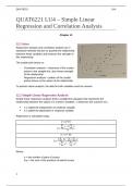
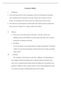
1. Bar Chart
X-axis (horizontal) represents categories
Y-axis (vertical) represents frequency counts or % of each category
The order of categories or widths of the bars don’t matter – only bar heights!!
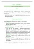
2. Pie Chart
A circle divided into category segments – size of each segments must be proportional to the
count of its category. Sum of the segment counts must equal 100%
Charts and graphs must have:
- Headings - Legends
- Axis titles - Data source
1
,QUAT6221 LU3
Two Categorical Variables Cross-tabulation Table / Contingency Table
= summarises the joint responses of two categorical variables. The table shows the number /
% of observations that jointly belong to each combination of categories of the 2 categorical
variables. This summary table is used to examine the association between 2 categorical
measures.
Steps to construct a cross-tabulation table:
- Prepare a table with m rows (m = the number of categories of the 1st variable) and n
column (n= the number of categories of the 2nd variable) = table with (m X n) cells.
- Assign each pair of data values from the two variables to an appropriate category
combination cell in the table by placing a tick in the relevant cell.
- When each pair of data values has been assigned to a cell in the table, count the
number of ticks per cell to derive the joint frequency count for each cell.
- Sum each row to give row totals per category of the row variable.
- Sum each column to give column totals per category of the column variable.
- Sum the column totals (or row totals) to give the grand total (sample size).
These joint frequency counts get converted to percentages - the percentages could be
expressed in terms of the total sample size or of row subtotals or of column subtotals.
A cross-tabulation/ contingency table can be displayed graphically as a:
- Stacked bar chart - Multiple bar chart
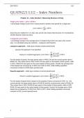
1. Stacked Bar Chart
Steps to construct:
- Choose the row variable and plot the frequency of each category of this variable as a
simple bar chart.
- Split the height of each bar in proportion to the frequency count of the categories of
the column variable.
This produces a simple bar chart of the row variable with each bar split proportionately into
the categories of the column variable. The categories of column variable are 'stacked' on top
of each other within each category bar of the row variable.
2. Multiple Bar Chart
Steps to construct:
- For each category of the row variable, plot a simple bar chart constructed from the
corresponding frequencies of the categories of the column variable.
- Display these categorised simple bar charts next to each other on the same axis
Similar to stacked bar chart, but stacked bars are next to each other rather than on top of
each other.
2.3 Summarising Numeric Data
Numeric data can be summarised in table format and displayed graphically – histogram
2
, QUAT6221 LU3
Single Numeric Variable – only 1
Numeric Frequency Distribution
= summarises numeric data into intervals of equal width. Each interval
shows how many numbers fall in the interval.
Steps to make:
- Determine data range
o Range = max data value – min data value
- Choose the number of intervals (k)
- Determine the interval width
o Interval width = data range / number of intervals
- Set up the interval limits.
- Tabulate the data values.
The frequency counts can be converted to % by dividing each frequency count by the
sample size. The resultant table is called a percentage or relative frequency distribution. It
shows the percentage of data values within each interval.
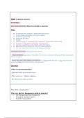
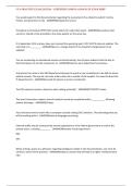
Histogram
= graphic display of a numeric frequency distribution
Steps:
- Arrange intervals consecutively on the x-axis from the lowest
interval to the highest (no gaps in-between adjacent interval limits)
- Plot the height of each bar on the y-axis over its corresponding
interval, to show either the frequency count or percentage frequency
of each interval. The area of a bar measures the density of values in
each interval
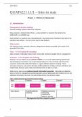
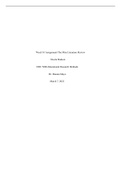
Cumulative Frequency Distribution
= summary table of cumulative frequency counts which is
used to answer questions of a ‘more than’ or ‘less than’
nature.
Steps to create a less than cumulative frequency
distribution from a numeric frequency distribution:
- For each interval, starting with the lowest interval, ask the question: 'How many data
values are below this interval's upper limit?'
- The answer is: the sum of all frequency counts (or percentages, or proportions) that
lie below this current interval's upper limit.
- This is repeated until the last interval is reached.
- The last interval's cumulative frequency count must always equal the sample size, n,
(or 100% or 1).
To find the more than cumulative frequency distribution, start from the highest interval’s
lower limit by asking the question: “how many data values are above this interval’s lower
3
QUAT6221 LU3 – Descriptive Statistics
Chapter 2 – Summarizing Data: Summary Tables and Graphs
2.2 Summarising Categorical Data
Single Categorical Variable
Categorical Frequency Table
= summarises data for a single categorical variable. Shows how many times each category
appears in a sample of data and measures the relative importance of the different
Steps to construct a categorical frequency table:
- List all categories of the variable – in 1st column
- Count and record the number of occurrences of each category – 2nd column
- Convert the counts per category into % of the total sample size. This produces a
percentage categorical frequency table – 3rd column
A categorical frequency table can be displayed graphically as a:
- Bar chart - Pie chart
Limitation of bar and pie chart = each displays the summarised info on only one variable at a
time.
1. Bar Chart
X-axis (horizontal) represents categories
Y-axis (vertical) represents frequency counts or % of each category
The order of categories or widths of the bars don’t matter – only bar heights!!
2. Pie Chart
A circle divided into category segments – size of each segments must be proportional to the
count of its category. Sum of the segment counts must equal 100%
Charts and graphs must have:
- Headings - Legends
- Axis titles - Data source
1
,QUAT6221 LU3
Two Categorical Variables Cross-tabulation Table / Contingency Table
= summarises the joint responses of two categorical variables. The table shows the number /
% of observations that jointly belong to each combination of categories of the 2 categorical
variables. This summary table is used to examine the association between 2 categorical
measures.
Steps to construct a cross-tabulation table:
- Prepare a table with m rows (m = the number of categories of the 1st variable) and n
column (n= the number of categories of the 2nd variable) = table with (m X n) cells.
- Assign each pair of data values from the two variables to an appropriate category
combination cell in the table by placing a tick in the relevant cell.
- When each pair of data values has been assigned to a cell in the table, count the
number of ticks per cell to derive the joint frequency count for each cell.
- Sum each row to give row totals per category of the row variable.
- Sum each column to give column totals per category of the column variable.
- Sum the column totals (or row totals) to give the grand total (sample size).
These joint frequency counts get converted to percentages - the percentages could be
expressed in terms of the total sample size or of row subtotals or of column subtotals.
A cross-tabulation/ contingency table can be displayed graphically as a:
- Stacked bar chart - Multiple bar chart
1. Stacked Bar Chart
Steps to construct:
- Choose the row variable and plot the frequency of each category of this variable as a
simple bar chart.
- Split the height of each bar in proportion to the frequency count of the categories of
the column variable.
This produces a simple bar chart of the row variable with each bar split proportionately into
the categories of the column variable. The categories of column variable are 'stacked' on top
of each other within each category bar of the row variable.
2. Multiple Bar Chart
Steps to construct:
- For each category of the row variable, plot a simple bar chart constructed from the
corresponding frequencies of the categories of the column variable.
- Display these categorised simple bar charts next to each other on the same axis
Similar to stacked bar chart, but stacked bars are next to each other rather than on top of
each other.
2.3 Summarising Numeric Data
Numeric data can be summarised in table format and displayed graphically – histogram
2
, QUAT6221 LU3
Single Numeric Variable – only 1
Numeric Frequency Distribution
= summarises numeric data into intervals of equal width. Each interval
shows how many numbers fall in the interval.
Steps to make:
- Determine data range
o Range = max data value – min data value
- Choose the number of intervals (k)
- Determine the interval width
o Interval width = data range / number of intervals
- Set up the interval limits.
- Tabulate the data values.
The frequency counts can be converted to % by dividing each frequency count by the
sample size. The resultant table is called a percentage or relative frequency distribution. It
shows the percentage of data values within each interval.
Histogram
= graphic display of a numeric frequency distribution
Steps:
- Arrange intervals consecutively on the x-axis from the lowest
interval to the highest (no gaps in-between adjacent interval limits)
- Plot the height of each bar on the y-axis over its corresponding
interval, to show either the frequency count or percentage frequency
of each interval. The area of a bar measures the density of values in
each interval
Cumulative Frequency Distribution
= summary table of cumulative frequency counts which is
used to answer questions of a ‘more than’ or ‘less than’
nature.
Steps to create a less than cumulative frequency
distribution from a numeric frequency distribution:
- For each interval, starting with the lowest interval, ask the question: 'How many data
values are below this interval's upper limit?'
- The answer is: the sum of all frequency counts (or percentages, or proportions) that
lie below this current interval's upper limit.
- This is repeated until the last interval is reached.
- The last interval's cumulative frequency count must always equal the sample size, n,
(or 100% or 1).
To find the more than cumulative frequency distribution, start from the highest interval’s
lower limit by asking the question: “how many data values are above this interval’s lower
3