lOMoARcPSD|51556245
Solutions Thomas Calculus 14th Edition [konkur
Information Security (Harper Adams University)
Scan to open on Studocu
Studocu is not sponsored or endorsed by any college or university
Downloaded by Lamsmmwaura Muiruri ()
, lOMoARcPSD|51556245
www.konkur.in
Thomas Calculus Early Transcendentals 14th Edition Hass SOLUTIONS
MANUAL
CHAPTER 2 LIMITS AND CONTINUITY
2.1 RATES OF CHANGE AND TANGENTS TO CURVES
f f (3)f (2) f f (1)f (1)
1. (a) x 32
289 19
1
(b) x 1(1) 20 2
1
g g (3) g (1) g g (4) g ( 2)
2. (a) x
3 1
3 (21) 2 (b) x
4 ( 2) 8 68 0
3. (a) h
h 34 h4 11 4 h 2h 6 0 3 3 3
(b) h
t 3 4 t
4 2 2 6 3
g g () g (0) (21)(21) g g () g () (21)(21)
4. (a) t 0
0
2
(b) t ( ) 2
0
5. R 20 81
R(2) R(0)
1 31
1
2 2
6. P 21
P (2) P (1) (81610)(145)
1
22 0
2 2
y
((2h ) 5)(2 5) 44h h 2 51 2
7. (a) x h
h
4h h 4 h. As h 0, 4 h 4 at P(2, 1) the slope is 4.
h
(b) y (1) 4( x 2) y 1 4 x 8 y 4 x 9
2 2
y
(7(2h )h )(72 ) 744hh h 3 4hh
2 2
8. (a) x h
4 h. As h 0, 4 h 4 at P(2, 3) the slope
is 4.
(b) y 3 (4)( x 2) y 3 4 x 8 y 4 x 11
y ((2h)2 2(2h)3)(22 2(2)3) 44h h 2 42h3(3) 2
9. (a) x h
h
2hh 2 h. As h 0, 2 h 2 at
h
P(2, 3) the slope is 2.
(b) y (3) 2( x 2) y 3 2 x 4 y 2x 7.
y ((1h) 4(1h))(1 4(1)) 12h h 44h(3)
2 2 2
10. (a) x h 2h h 2. As h 0, h 2 2 at P(1, 3) the
2
h
h h
slope is 2.
(b) y (3) (2)( x 1) y 3 2 x 2 y 2x 1.
Downloaded by Lamsmmwaura Muiruri ()
forum.konkur.in
, lOMoARcPSD|51556245
www.konkur.in
y (2h)3 23 h 8 12h 4h h 12 4h h 2 . As h 0, 12 4h h 2 12, at P(2, 8)
2 3 2 3
11. (a) x h
812h 4h
h h
the slope is 12.
(b) y 8 12( x 2) y 8 12 x 24 y 12x 16.
y 2(1 h)3 (213 )
213h3h h 1 3h3h h 3 3h h 2 . As h 0, 3 3h h 2 3, at
2 3 2 3
12. (a) x h h h
P(1, 1) the slope is 3.
(b) y 1 (3)( x 1) y 1 3x 3 y 3x 4.
Copyright 2018 Pearson Education, Inc.
61
Downloaded by Lamsmmwaura Muiruri ()
forum.konkur.in
, lOMoARcPSD|51556245
www.konkur.in
62 Chapter 2 Limits and Continuity
62
y (1h) 12(1h)(1 12(1)) 13h3h h 1212h(11)
3 3 2 3
13. (a) x 9h3h h 9 3h h 2 .
2 3
h h h
As h 0, 9 3h h 2 9 at P(1, 11) the slope is 9.
(b) y (11) (9)( x 1) y 11 9 x 9 y 9x 2.
y (2h) 3(2h) 4(2 3(2) 4)
3 2 3 2
812h 6h h 1212h 3h 40 3h h 3h h2 .
2 3 2 2 3
14. (a) x h h h
As h 0, 3h h 2 0 at P(2, 0) the slope is 0.
(b) y 0 0( x 2) y 0.
y
1 2
1
2(2h)
15. (a) x
2hh 2(2h) h1 2(2h)
1 .
As h 0, 2(2
1 41 , at P 2, 1
the slope is 1 .
h) 2 4
(b) y 1 1 ( x (2)) y 1 1 x 1 y 1 x 1
2 4 2 4 2 4
(4h )
24
4
y 4 h 2 1 4h2(2h) 1 1 1 .
2h
2(4h )
16. (a) x 1 h h 2h 2h
h 2 h
As h 0, 21 h 12 , at P(4, 2) the slope is 12 .
(b) y (2) 12 ( x 4) y 2 12 x 2 y 12 x 4
y
4hh 4 4hh 2 4h 2
(4 h)4
17. (a) 1 .
x 4h 2 h( 4h 2) 4h 2
As h 0, 1 1 1, at P(4, 2) the slope is 14 .
4h 2 4 2 4
(b) y 2 14 ( x 4) y 2 14 x 1 y 14 x 1
y 7(2h) 7(2) 3 3 9h 3 (9h)9 1
18. (a) x
9h 9h .
h h h 9h 3 h( 9h 3) 9h 3
As h 0, 1 1 1 , at P(2, 3) the slope is 1 .
9h 3 9 3 6 6
(b) y 3 1 ( x (2)) y 3 1 x 1 y 1 x 8
6 6 3 6 3
p
19. (a) Q Slope of PQ
t
Q1 (10, 225) 650225
2010
42.5 m/sec
Q2 (14, 375) 650375
2014 45.83 m/sec
Q3 (16.5, 475) 650475
50.00 m/sec
2016.5
Q4 (18, 550) 650550
2018
50.00 m/sec
(b) At t 20, the sportscar was traveling approximately 50 m/sec or 180 km/h.
p
20. (a) Q Slope of PQ t
Q1 (5, 20) 8020 12 m/sec
105
107 13.7 m/sec
Q2 (7, 39) 8039
Q3 (8.5, 58) 8058
14.7 m/sec
108.5
Q4 (9.5, 72) 8072
109.5
16 m/sec
(b) Approximately 16 m/sec
Copyright 2018 Pearson Education, Inc.
Downloaded by Lamsmmwaura Muiruri ()
forum.konkur.in
, lOMoARcPSD|51556245
www.konkur.in
Section 2.1 Rates of Change and Tangents to Curves 63
21. (a)
p
200
Profit (1000s)
160
120
80
40
0 t
2010 2011 2012 2013 2014
Ye ar
p 17462
(b) t
20142012 112
2
56 thousand dollars per year
(c) The average rate of change from 2011 to 2012 is p
t
20122011
6227 35 thousand dollars per year.
p
The average rate of change from 2012 to 2013 is t 20132012
11162 49 thousand dollars per year.
So, the rate at which profits were changing in 2012 is approximately 12 (35 49) 42 thousand dollars
per year.
22. (a) F ( x) ( x 2)/( x 2)
x 1.2 1.1 1.01 1.001 1.0001 1
F ( x) 4.0 3.4 3.04 3.004 3.0004 3
F 4.0(3) F 3.4 (3)
x
5.0; 1.21
4.4; x 1.11
F 3.04(3) 4.04; F 3.004(3) 4.004;
x 1.011 x 1.0011
F
x
3.0004(3) 4.0004;
1.00011
(b) The rate of change of F ( x ) at x 1 is 4.
g g (2) g (1) g g (1.5) g (1) 1
23. (a) x 21
21
21
0.414213 x
1.51
1.5
0.5
0.449489
g g (1h) g (1) 1
x (1h)1
1hh
(b) g ( x) x
1 h 1.1 1.01 1.001 1.0001 1.00001 1.000001
1 h 1.04880 1.004987 1.0004998 1.0000499 1.000005 1.0000005
1 h 1 /h 0.4880 0.4987 0.4998 0.499 0.5 0.5
(c) The rate of change of g ( x ) at x 1 is 0.5.
1 1
(d) The calculator gives lim 1h
h
2.
h0
11 1
f (3)f (2)
24. (a) i) 3 1 2 16 61
32
1 1 2 T
f(T)f (2)
ii) TT 22 2TT 2
T 2
2T
2T2T 2T 2T
(T 2) 2T (2T )
1 ,T 2
(b) T 2.1 2.01 2.001 2.0001 2.00001 2.000001
f (T ) 0.476190 0.497512 0.499750 0.4999750 0.499997 0.499999
( f (T ) f (2))/(T 2) 0.2381 0.2488 0.2500 0.2500 0.2500 0.2500
(c) The table indicates the rate of change is 0.25 at t 2.
(d) lim 1 1
T 2 2T 4
NOTE: Answers will vary in Exercises 25 and 26.
25. (a) [0, 1]: s 150 15 mph; [1, 2.5]: s 2015 10 mph; [2.5, 3.5]: s 3020 10 mph
t 10 t 2.51 3 t 3.52.5
Copyright 2018 Pearson Education, Inc.
Downloaded by Lamsmmwaura Muiruri ()
forum.konkur.in
, lOMoARcPSD|51556245
www.konkur.in
64 Chapter 2 Limits and Continuity Section 2.2 Limit of a Function and Limit Laws 64
64 64
2
(b) At P 1 , 7.5 : Since the portion of the graph from t 0 to t 1 is nearly linear, the instantaneous rate of
change will be almost the same as the average rate of change, thus the instantaneous speed at t 12 is
157.5 15 mi/hr. At P(2, 20): Since the portion of the graph from t 2 to t 2.5 is nearly linear, the
10.5
instantaneous rate of change will be nearly the same as the average rate of change, thus v 2020
2.52 0 mi/hr.
For values of t less than 2, we have
s
Slope of PQ t
Q
Q1 (1, 15) 1520 5 mi/hr
12
Q2 (1.5, 19) 1920
1.52
2 mi/hr
19.920
Q3 (1.9, 19.9)
1.92
1 mi/hr
Thus, it appears that the instantaneous speed at t 2 is 0 mi/hr.
At P(3, 22):
s
Slope of PQ t Q Slope of PQ s
Q t
Q1 (2, 20) 2022
Q1 (4, 35) 3522
43
13 mi/hr 23
2 mi/hr
Q2 (3.5, 30) 3022
16 mi/hr Q2 (2.5, 20) 2022
2.53
4 mi/hr
3.53
21.622
Q3 (3.1, 23) 2322 10 mi/hr Q3 (2.9, 21.6) 4 mi/hr
3.13 2.93
Thus, it appears that the instantaneous speed at t 3 is about 7 mi/hr.
(c) It appears that the curve is increasing the fastest at t 3.5. Thus for P (3.5, 30)
s
Slope of PQ t
Q Q Slope of PQ s
t
Q1 (4, 35) 3530 10 mi/hr 2230 16 mi/hr
43.5 Q1 (3, 22)
33.5
Q2 (3.75, 34) 3430
3.753.5
16 mi/hr Q2 (3.25, 25) 2530
20 mi/hr
3.253.5
Q3 (3.6, 32) 3230
3.63.5
20 mi/hr Q3 (3.4, 28) 2830
20 mi/hr
3.43.5
Thus, it appears that the instantaneous speed at t 3.5 is about 20 mi/hr.
26. (a) [0, 3]: tA 1015 1.67 day ; [0, 5]: tA 3.915 2.2 day; [7, 10]: t
gal gal
A 01.4 0.5 gal
30 50 107 day
(b) At P(1, 14) :
A
Q Slope of PQ t Q Slope of PQ tA
Q1 (2, 12.2) 12.214 1.8 gal/day Q1 (0, 15) 1514 1 gal/day
21 01
Q2 (1.5, 13.2) 13.214 14.614
1.51
1.6 gal/day Q2 (0.5, 14.6) 1.2 gal/day
0.51
Q3 (1.1, 13.85) 13.8514 1.5 gal/day
1.11
Q3 (0.9, 14.86) 14.8614 1.4 gal/day
0.91
Thus, it appears that the instantaneous rate of consumption at t 1 is about 1.45 gal/day.
At P(4, 6):
Q Slope of PQ tA
Q Slope of PQ tA
Q (5, 3.9)
1
3.96 2.1 gal/day Q1 (3, 10) 106
4 gal/day34
54
Q2 (4.5, 4.8) 4.86
2.4 gal/day Q2 (3.5, 7.8) 7.86
3.54
3.6 gal/day
4.54
Q3 (4.1, 5.7) 5.76
3 gal/day Q3 (3.9, 6.3) 6.36
3.94
3 gal/day
4.14
Thus, it appears that the instantaneous rate of consumption at t 1 is 3 gal/day.
(solution continues on next page)
Copyright 2018 Pearson Education, Inc.
Downloaded by Lamsmmwaura Muiruri ()
forum.konkur.in
Solutions Thomas Calculus 14th Edition [konkur
Information Security (Harper Adams University)
Scan to open on Studocu
Studocu is not sponsored or endorsed by any college or university
Downloaded by Lamsmmwaura Muiruri ()
, lOMoARcPSD|51556245
www.konkur.in
Thomas Calculus Early Transcendentals 14th Edition Hass SOLUTIONS
MANUAL
CHAPTER 2 LIMITS AND CONTINUITY
2.1 RATES OF CHANGE AND TANGENTS TO CURVES
f f (3)f (2) f f (1)f (1)
1. (a) x 32
289 19
1
(b) x 1(1) 20 2
1
g g (3) g (1) g g (4) g ( 2)
2. (a) x
3 1
3 (21) 2 (b) x
4 ( 2) 8 68 0
3. (a) h
h 34 h4 11 4 h 2h 6 0 3 3 3
(b) h
t 3 4 t
4 2 2 6 3
g g () g (0) (21)(21) g g () g () (21)(21)
4. (a) t 0
0
2
(b) t ( ) 2
0
5. R 20 81
R(2) R(0)
1 31
1
2 2
6. P 21
P (2) P (1) (81610)(145)
1
22 0
2 2
y
((2h ) 5)(2 5) 44h h 2 51 2
7. (a) x h
h
4h h 4 h. As h 0, 4 h 4 at P(2, 1) the slope is 4.
h
(b) y (1) 4( x 2) y 1 4 x 8 y 4 x 9
2 2
y
(7(2h )h )(72 ) 744hh h 3 4hh
2 2
8. (a) x h
4 h. As h 0, 4 h 4 at P(2, 3) the slope
is 4.
(b) y 3 (4)( x 2) y 3 4 x 8 y 4 x 11
y ((2h)2 2(2h)3)(22 2(2)3) 44h h 2 42h3(3) 2
9. (a) x h
h
2hh 2 h. As h 0, 2 h 2 at
h
P(2, 3) the slope is 2.
(b) y (3) 2( x 2) y 3 2 x 4 y 2x 7.
y ((1h) 4(1h))(1 4(1)) 12h h 44h(3)
2 2 2
10. (a) x h 2h h 2. As h 0, h 2 2 at P(1, 3) the
2
h
h h
slope is 2.
(b) y (3) (2)( x 1) y 3 2 x 2 y 2x 1.
Downloaded by Lamsmmwaura Muiruri ()
forum.konkur.in
, lOMoARcPSD|51556245
www.konkur.in
y (2h)3 23 h 8 12h 4h h 12 4h h 2 . As h 0, 12 4h h 2 12, at P(2, 8)
2 3 2 3
11. (a) x h
812h 4h
h h
the slope is 12.
(b) y 8 12( x 2) y 8 12 x 24 y 12x 16.
y 2(1 h)3 (213 )
213h3h h 1 3h3h h 3 3h h 2 . As h 0, 3 3h h 2 3, at
2 3 2 3
12. (a) x h h h
P(1, 1) the slope is 3.
(b) y 1 (3)( x 1) y 1 3x 3 y 3x 4.
Copyright 2018 Pearson Education, Inc.
61
Downloaded by Lamsmmwaura Muiruri ()
forum.konkur.in
, lOMoARcPSD|51556245
www.konkur.in
62 Chapter 2 Limits and Continuity
62
y (1h) 12(1h)(1 12(1)) 13h3h h 1212h(11)
3 3 2 3
13. (a) x 9h3h h 9 3h h 2 .
2 3
h h h
As h 0, 9 3h h 2 9 at P(1, 11) the slope is 9.
(b) y (11) (9)( x 1) y 11 9 x 9 y 9x 2.
y (2h) 3(2h) 4(2 3(2) 4)
3 2 3 2
812h 6h h 1212h 3h 40 3h h 3h h2 .
2 3 2 2 3
14. (a) x h h h
As h 0, 3h h 2 0 at P(2, 0) the slope is 0.
(b) y 0 0( x 2) y 0.
y
1 2
1
2(2h)
15. (a) x
2hh 2(2h) h1 2(2h)
1 .
As h 0, 2(2
1 41 , at P 2, 1
the slope is 1 .
h) 2 4
(b) y 1 1 ( x (2)) y 1 1 x 1 y 1 x 1
2 4 2 4 2 4
(4h )
24
4
y 4 h 2 1 4h2(2h) 1 1 1 .
2h
2(4h )
16. (a) x 1 h h 2h 2h
h 2 h
As h 0, 21 h 12 , at P(4, 2) the slope is 12 .
(b) y (2) 12 ( x 4) y 2 12 x 2 y 12 x 4
y
4hh 4 4hh 2 4h 2
(4 h)4
17. (a) 1 .
x 4h 2 h( 4h 2) 4h 2
As h 0, 1 1 1, at P(4, 2) the slope is 14 .
4h 2 4 2 4
(b) y 2 14 ( x 4) y 2 14 x 1 y 14 x 1
y 7(2h) 7(2) 3 3 9h 3 (9h)9 1
18. (a) x
9h 9h .
h h h 9h 3 h( 9h 3) 9h 3
As h 0, 1 1 1 , at P(2, 3) the slope is 1 .
9h 3 9 3 6 6
(b) y 3 1 ( x (2)) y 3 1 x 1 y 1 x 8
6 6 3 6 3
p
19. (a) Q Slope of PQ
t
Q1 (10, 225) 650225
2010
42.5 m/sec
Q2 (14, 375) 650375
2014 45.83 m/sec
Q3 (16.5, 475) 650475
50.00 m/sec
2016.5
Q4 (18, 550) 650550
2018
50.00 m/sec
(b) At t 20, the sportscar was traveling approximately 50 m/sec or 180 km/h.
p
20. (a) Q Slope of PQ t
Q1 (5, 20) 8020 12 m/sec
105
107 13.7 m/sec
Q2 (7, 39) 8039
Q3 (8.5, 58) 8058
14.7 m/sec
108.5
Q4 (9.5, 72) 8072
109.5
16 m/sec
(b) Approximately 16 m/sec
Copyright 2018 Pearson Education, Inc.
Downloaded by Lamsmmwaura Muiruri ()
forum.konkur.in
, lOMoARcPSD|51556245
www.konkur.in
Section 2.1 Rates of Change and Tangents to Curves 63
21. (a)
p
200
Profit (1000s)
160
120
80
40
0 t
2010 2011 2012 2013 2014
Ye ar
p 17462
(b) t
20142012 112
2
56 thousand dollars per year
(c) The average rate of change from 2011 to 2012 is p
t
20122011
6227 35 thousand dollars per year.
p
The average rate of change from 2012 to 2013 is t 20132012
11162 49 thousand dollars per year.
So, the rate at which profits were changing in 2012 is approximately 12 (35 49) 42 thousand dollars
per year.
22. (a) F ( x) ( x 2)/( x 2)
x 1.2 1.1 1.01 1.001 1.0001 1
F ( x) 4.0 3.4 3.04 3.004 3.0004 3
F 4.0(3) F 3.4 (3)
x
5.0; 1.21
4.4; x 1.11
F 3.04(3) 4.04; F 3.004(3) 4.004;
x 1.011 x 1.0011
F
x
3.0004(3) 4.0004;
1.00011
(b) The rate of change of F ( x ) at x 1 is 4.
g g (2) g (1) g g (1.5) g (1) 1
23. (a) x 21
21
21
0.414213 x
1.51
1.5
0.5
0.449489
g g (1h) g (1) 1
x (1h)1
1hh
(b) g ( x) x
1 h 1.1 1.01 1.001 1.0001 1.00001 1.000001
1 h 1.04880 1.004987 1.0004998 1.0000499 1.000005 1.0000005
1 h 1 /h 0.4880 0.4987 0.4998 0.499 0.5 0.5
(c) The rate of change of g ( x ) at x 1 is 0.5.
1 1
(d) The calculator gives lim 1h
h
2.
h0
11 1
f (3)f (2)
24. (a) i) 3 1 2 16 61
32
1 1 2 T
f(T)f (2)
ii) TT 22 2TT 2
T 2
2T
2T2T 2T 2T
(T 2) 2T (2T )
1 ,T 2
(b) T 2.1 2.01 2.001 2.0001 2.00001 2.000001
f (T ) 0.476190 0.497512 0.499750 0.4999750 0.499997 0.499999
( f (T ) f (2))/(T 2) 0.2381 0.2488 0.2500 0.2500 0.2500 0.2500
(c) The table indicates the rate of change is 0.25 at t 2.
(d) lim 1 1
T 2 2T 4
NOTE: Answers will vary in Exercises 25 and 26.
25. (a) [0, 1]: s 150 15 mph; [1, 2.5]: s 2015 10 mph; [2.5, 3.5]: s 3020 10 mph
t 10 t 2.51 3 t 3.52.5
Copyright 2018 Pearson Education, Inc.
Downloaded by Lamsmmwaura Muiruri ()
forum.konkur.in
, lOMoARcPSD|51556245
www.konkur.in
64 Chapter 2 Limits and Continuity Section 2.2 Limit of a Function and Limit Laws 64
64 64
2
(b) At P 1 , 7.5 : Since the portion of the graph from t 0 to t 1 is nearly linear, the instantaneous rate of
change will be almost the same as the average rate of change, thus the instantaneous speed at t 12 is
157.5 15 mi/hr. At P(2, 20): Since the portion of the graph from t 2 to t 2.5 is nearly linear, the
10.5
instantaneous rate of change will be nearly the same as the average rate of change, thus v 2020
2.52 0 mi/hr.
For values of t less than 2, we have
s
Slope of PQ t
Q
Q1 (1, 15) 1520 5 mi/hr
12
Q2 (1.5, 19) 1920
1.52
2 mi/hr
19.920
Q3 (1.9, 19.9)
1.92
1 mi/hr
Thus, it appears that the instantaneous speed at t 2 is 0 mi/hr.
At P(3, 22):
s
Slope of PQ t Q Slope of PQ s
Q t
Q1 (2, 20) 2022
Q1 (4, 35) 3522
43
13 mi/hr 23
2 mi/hr
Q2 (3.5, 30) 3022
16 mi/hr Q2 (2.5, 20) 2022
2.53
4 mi/hr
3.53
21.622
Q3 (3.1, 23) 2322 10 mi/hr Q3 (2.9, 21.6) 4 mi/hr
3.13 2.93
Thus, it appears that the instantaneous speed at t 3 is about 7 mi/hr.
(c) It appears that the curve is increasing the fastest at t 3.5. Thus for P (3.5, 30)
s
Slope of PQ t
Q Q Slope of PQ s
t
Q1 (4, 35) 3530 10 mi/hr 2230 16 mi/hr
43.5 Q1 (3, 22)
33.5
Q2 (3.75, 34) 3430
3.753.5
16 mi/hr Q2 (3.25, 25) 2530
20 mi/hr
3.253.5
Q3 (3.6, 32) 3230
3.63.5
20 mi/hr Q3 (3.4, 28) 2830
20 mi/hr
3.43.5
Thus, it appears that the instantaneous speed at t 3.5 is about 20 mi/hr.
26. (a) [0, 3]: tA 1015 1.67 day ; [0, 5]: tA 3.915 2.2 day; [7, 10]: t
gal gal
A 01.4 0.5 gal
30 50 107 day
(b) At P(1, 14) :
A
Q Slope of PQ t Q Slope of PQ tA
Q1 (2, 12.2) 12.214 1.8 gal/day Q1 (0, 15) 1514 1 gal/day
21 01
Q2 (1.5, 13.2) 13.214 14.614
1.51
1.6 gal/day Q2 (0.5, 14.6) 1.2 gal/day
0.51
Q3 (1.1, 13.85) 13.8514 1.5 gal/day
1.11
Q3 (0.9, 14.86) 14.8614 1.4 gal/day
0.91
Thus, it appears that the instantaneous rate of consumption at t 1 is about 1.45 gal/day.
At P(4, 6):
Q Slope of PQ tA
Q Slope of PQ tA
Q (5, 3.9)
1
3.96 2.1 gal/day Q1 (3, 10) 106
4 gal/day34
54
Q2 (4.5, 4.8) 4.86
2.4 gal/day Q2 (3.5, 7.8) 7.86
3.54
3.6 gal/day
4.54
Q3 (4.1, 5.7) 5.76
3 gal/day Q3 (3.9, 6.3) 6.36
3.94
3 gal/day
4.14
Thus, it appears that the instantaneous rate of consumption at t 1 is 3 gal/day.
(solution continues on next page)
Copyright 2018 Pearson Education, Inc.
Downloaded by Lamsmmwaura Muiruri ()
forum.konkur.in